1  Introduction to R

Abstract

In this chapter, we introduce six key concepts for data analysis. We subsequently describe the R programming language and RStudio, its most popular Integrated Development Environment. Finally, we share key foundational concepts when programming with R.

1.1 Six Principles for Data Analysis

1.1.1 Accuracy

Deliberate steps should be taken to minimize the chance of making an error and maximize the chance of catching errors when errors inevitably occur. ¹

1.1.2 Computational reproducibility

Computational reproducibility should be embraced to improve accuracy, promote transparency, and prove the quality of analytic work.

Replication: the recreation of findings across repeated studies, is a cornerstone of science.

Reproducibility: the ability to access data, source code, tools, and documentation and recreate all calculations, visualizations, and artifacts of an analysis.

Computational reproducibility should be the minimum standard for computational social sciences and statistical programming.

1.1.3 Human interpretability

Code should be written so humans can easily understand what’s happening—even if it occasionally sacrifices machine performance.

1.1.4 Portability

Analyses should be designed so strangers can understand each and every step without additional instruction or inquiry from the original analyst.

1.1.5 Accessibility

Research and data are non-rivalrous and can be non-excludable. They are public goods that should be widely and easily shared. Decisions about tools, methods, data, and language during the research process should be made in ways that promote the ability of anyone and everyone to access an analysis.

1.1.6 Efficiency

Analysts should seek to make all parts of the research process more efficient with clear communication, by adopting best practices, and by managing computation.

1.2 R

R is a free, open-source software for statistical computing. It is a fully-functioning programming language and it is known for intuitive, crisp graphics and an extensive, growing library of statistical and analytic methods. Above all, R boasts an enthusiastic community of developers, instructors, and users. The copyright and documentation for R is held by a not-for-profit organization called the R Foundation.

R comes from the S programming language and S-PLUS system. In addition to offering better graphics and more extensibility than proprietary languages, R has a pedagogical advantage:

The ambiguity [of the S language] is real and goes to a key objective: we wanted users to be able to begin in an interactive environment, where they did not consciously think of themselves as programming. Then as their needs became clearer and their sophistication increased, they should be able to slide gradually into programming, when the language and system aspects would become more important.

Source: Peng (2018)

1.3 RStudio

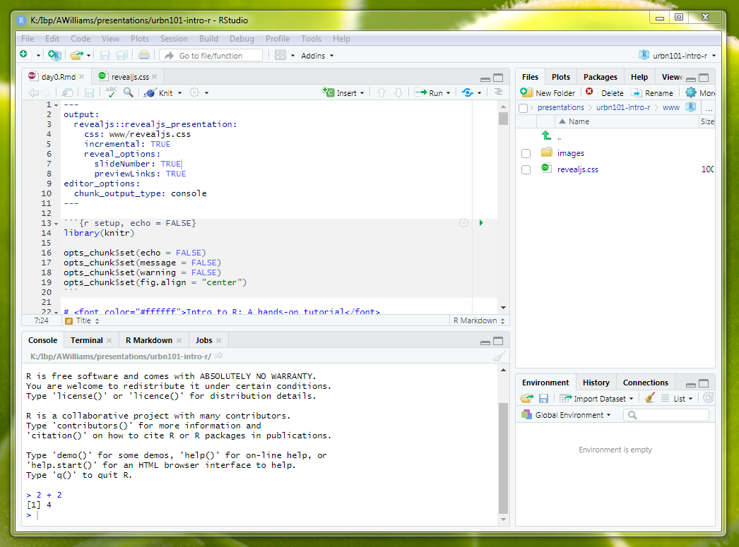
RStudio is a free, open-source integrated development environment (IDE) that runs on top of R. In practice, R users almost exclusively open RStudio and rarely directly open R. When we say IDE, we mean a piece of software where you can write, or develop, code in an efficient way.

RStudio is developed by a for-profit company called Posit. Posit used to be called RStudio. Posit employs some of the R community’s most prolific, open-source developers and creates many open-source tools and resources. ²

While R code can be written in any text editor, the RStudio IDE is a powerful tool with a console, syntax-highlighting, and debugging tools. The RStudio IDE cheatsheet outlines some of the power of RStudio.

1.4 RStudio Console

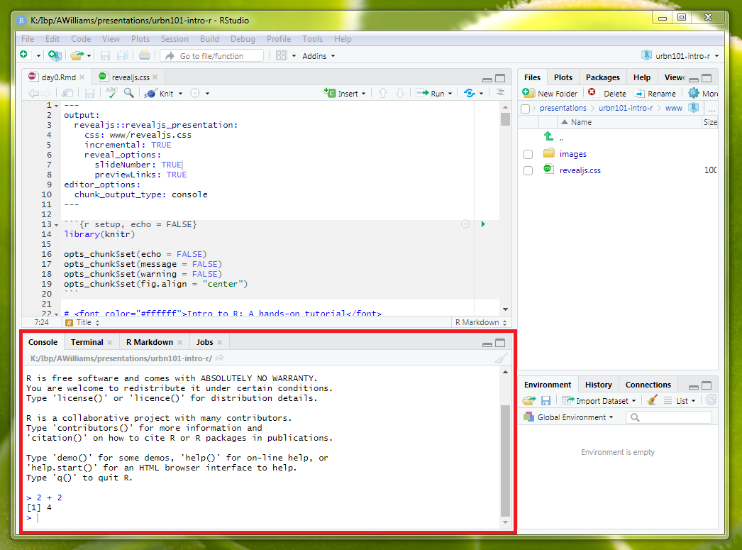
The RStudio Console contains the R command line and R output from previously submitted R code.

Code can be submitted by typing to the right of the last blue > and the hitting enter.

Exercise 1

R has all of the functionality of a basic calculator. Let’s run some simple calculations with addition (+), subtraction (-), multiplication (*), division (/), exponentiation (^), and grouping (()).

1.5 .R Scripts

By default, there isn’t a record of code directly typed and submitted into the RStudio Console. So, most R programmers use .R scripts to develop R code before submitting code to the console.

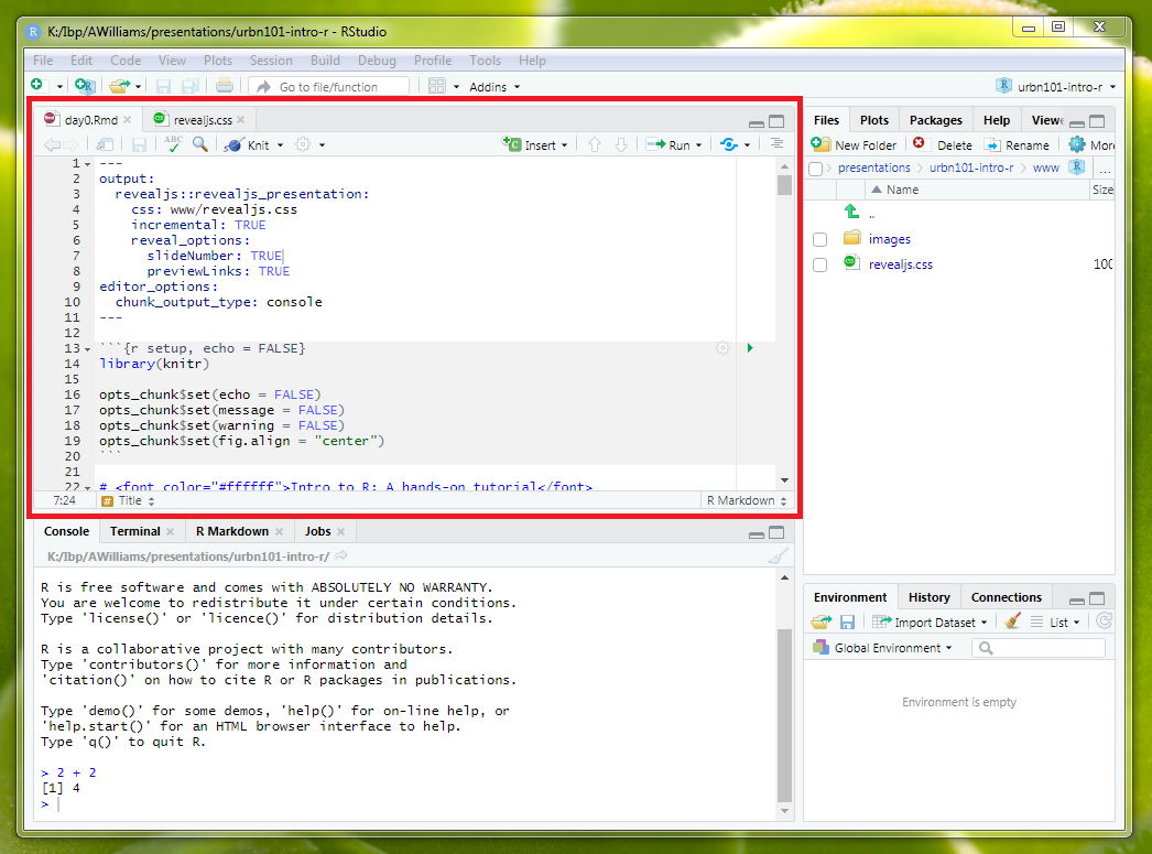
.R scripts are simple text files with R code. They are similar to .py files in Python, .sas files in SAS, and .do files in Stata.

Exercise 2

Click the new script button in the top left corner of RStudio to create a new script.

Add some R code to your new script. Place your cursor on a line of R code and hit Command-Enter on Macs or Control-Enter on Windows. Alternatively, highlight the code (it can be multiple lines) and click the run button.

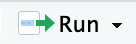
In both cases, the code from your .R script should move to the R Console and evaluate.

1.6 Comments

R will interpret all text in a .R script as R code unless the code follows #, the comment symbol. Comments are essential to writing clear code in any programming language.

## Demonstrate the value of a comment and make a simple calculation
2 + 2

It should be obvious what a line of clear R code accomplishes. It isn’t always obvious why a clear line of R code is included in a script. Comments should focus on the why of R code and not the what of R code.

The following comment isn’t useful because it just restates the R code, which is clear:

# divide every value by 1.11
cost / 1.11

The following comment is useful because it adds context to the R code:

# convert costs from dollars to Euros using the 2020-01-13 exchange rate
cost / 1.11

Exercise 3

Add comments to your .R that clarify the why. Since we only know a few operations, the comments may need to focus on your why you picked your favorite numbers.

1.7 Style

Good coding style is like correct punctuation: you can manage without it, butitsuremakesthingseasiertoread. ~ Wickham (n.d.)

Human interpretability is one of the six principles because clear code can save time and reduce the chance of making errors. After time, eyes can be trained to quickly spot incorrect code if a consistent R style is adopted.

First, note that R is case-sensitive. Capitalization is rare and deviations from the capitalization will throw errors. For example, mean() is a function but Mean() is not a function.

The tidyverse style guide is a comprehensive style guide that, in general, reflects the style of the plurality of R programmers. For now, just focus on consistency.

1.8 Data Structures

Data analysis is not possible without data structures for data. R has several important data structures that shape how information is stored and processed.

1.8.1 Vectors

Vectors are one-dimensional arrays that contain one and only one type of data. Atomic vectors in R are homogeneous. There are six types of atomic vectors:

• logical
• integer
• double
• character
• complex (uncommon)
• raw (uncommon)

For now, the simplest way to create a vector is with c(), the combine function.

# a logical vector
c(TRUE, FALSE, FALSE)

[1]  TRUE FALSE FALSE

# an integer vector
c(1, 2, 3)

[1] 1 2 3

# a double vector
c(1.1, 2.2, 3.3)

[1] 1.1 2.2 3.3

# a character vector
c("District of Columbia", "Virginia", "Maryland")

[1] "District of Columbia" "Virginia"             "Maryland"            

The class() function can be used to identify the type, or class, of an object. For example:

class(c(TRUE, FALSE, FALSE))

[1] "logical"

class(c(1, 2, 3))

[1] "numeric"

class(c("District of Columbia", "Virginia", "Maryland"))

[1] "character"

If you create a vector with mixed data types, R will coerce all of the values to a single type:

c(TRUE, 1, "District of Columbia")

[1] "TRUE"                 "1"                    "District of Columbia"

class(c(TRUE, 1, "District of Columbia"))

[1] "character"

Lists are one- or multi-dimensional arrays that are made up of other lists. Lists are heterogeneous - they can contain many lists of different types and dimensions. A vector is a list but a list is not necessarily a vector.

NULL is the null object in R. It means a value does not exist.

NA is a missing value of length 1 in R. NAs are powerful representations in R with special properties. NA is a contagious value in R that will override all calculations (Wickham and Grolemund 2017, sec. 20.2).

1 + 2 + 3 + NA

[1] NA

This forces programmers to be deliberate about missing values. This is a feature, not a bug!

R contains special functions and function arguments for handling NAs. For example, we can wrap a vector with missing values in is.na() to create a vector of Booleans where TRUE represents an element that is an NA and FALSE represents an element that is not an NA.

is.na(c(1, 2, NA))

[1] FALSE FALSE  TRUE

Note: NA and NULL have different meanings! NULL means no value exists. NA means a value could exist but it is unknown.

1.8.2 Matrices

Matrices are multi-dimensional arrays where every element is of the same type. Most data in data science contains at least numeric information and character information. Accordingly, we will not use matrices much in this course.

1.8.3 Data frames

Instead, data frames, and their powerful cousins tibbles, are the backbone of data science and this course. Data frames are two-dimensional arrays where each column is a list (usually a vector). Most times, each column will be of one type while a given row will contain many different types. We usually refer to columns as variables and rows as observations.

Here are the first six rows of a data frame with information about diamond prices and diamond characteristics:

head(ggplot2::diamonds)

# A tibble: 6 × 10
  carat cut       color clarity depth table price     x     y     z
  <dbl> <ord>     <ord> <ord>   <dbl> <dbl> <int> <dbl> <dbl> <dbl>
1  0.23 Ideal     E     SI2      61.5    55   326  3.95  3.98  2.43
2  0.21 Premium   E     SI1      59.8    61   326  3.89  3.84  2.31
3  0.23 Good      E     VS1      56.9    65   327  4.05  4.07  2.31
4  0.29 Premium   I     VS2      62.4    58   334  4.2   4.23  2.63
5  0.31 Good      J     SI2      63.3    58   335  4.34  4.35  2.75
6  0.24 Very Good J     VVS2     62.8    57   336  3.94  3.96  2.48

1.8.4 tibbles

tibbles are special data frames that have a few extra features:

• Only the first ten rows of tibbles print by default
• Extra meta data are printed with tibbles
• They have some convenient protections against partial subsetting (Wickham, Çetinkaya-Rundel, and Grolemund 2023, sec. 3.1.2)
• They are easier to create from scratch in a .R script

tibble(
  a = c(TRUE, FALSE, FALSE),
  b = c(1, 2, 3),
  c = c(1.1, 2.2, 3.3),
  d = c("District of Columbia", "Virginia", "Maryland")
)

# A tibble: 3 × 4
  a         b     c d                   
  <lgl> <dbl> <dbl> <chr>               
1 TRUE      1   1.1 District of Columbia
2 FALSE     2   2.2 Virginia            
3 FALSE     3   3.3 Maryland            

From this moment forward, I will use data frame to mean tibble.

1.9 Assignment

R can operate on many different vectors and data frames in the same R session. This creates much flexibility. It also means most unique objects in an R session need unique names.

<- is the assignment operator. An object created on the right side of an assignment operator is assigned to a name on the left side of an assignment operator. Assignment operators are important for saving the consequences of operations and functions. Without assignment, the result of a calculation is not saved for use in a future calculation. Operations without assignment operators will typically be printed to the console but not saved for future use.

# this important calculation is saved to the R environment
important_calculation <- 2 + 2

# this important calculation is NOT saved to the R environment
2 + 2

[1] 4

Style note: Objects should be given names that are “concise and meaningful” (Wickham, n.d., sec. 2). Generally the names should be nouns and only use lowercase letters, numbers, and underscores _ (this is referred to as snake case).

Exercise 4

Write three arithmetic operations in R and assign them to unique names. Then perform arithmetic operations using the named results. For example:

a <- 5 + 5 + 5
b <- 6 - 6 - 6

a + b

[1] 9

1.10 Functions

+, -, *, and / are great, but data science requires a lot more than just basic arithmetic.

R contains many more functions that can perform mathematical operations, control your computer operating system, process text data, and more. In fact, R is built around functions.

Because R was developed by statisticians, R’s functions have a lot in common with mathematical functions.

• Functions have inputs and outputs
• Each input has one and only one output (unless is involves a random process)

Functions are recognizable because they end in (). For example, the following calculates the mean of a numeric vector two ways:

mean(x = c(1, 2, 3))

[1] 2

numeric_vector <- c(1, 2, 3)
mean(x = numeric_vector)

[1] 2

Modern R with the tidyverse (Rodrigues 2022) has a functional programming chapter that contains more information about functional programming in R.

1.10.1 ?

Documentation for functions can be easily accessed by prefacing the function name with ? and dropping the ().

?mean

The documentation typically includes a description, a list of the arguments, references, a list of related functions, and examples. The examples are incredibly useful.

1.10.2 Arguments

R functions typically contain many arguments. For example, mean() has x, trim, and na.rm. Many arguments have default values and don’t need to be included in function calls. Default values can be seen in the documentation. trim = 0 and na.rm = FALSE are the defaults for mean().

Arguments can be passed to functions implicitly by position or explicitly by name.

numeric_vector <- c(1, 2, 3, 4, 5, 6, 7, 8, 9, 10)

# by position (correctly)
mean(numeric_vector, 0.2)

[1] 5.5

# by position (incorrectly)
mean(0.2, numeric_vector)

# by name
mean(x = numeric_vector, trim = 0.2)

[1] 5.5

Function calls can include arguments by position and by name. The first argument in most functions is data or x. It is custom to usually include the first argument by position and then all subsequent arguments by name.

mean(numeric_vector, trim = 0.2)

[1] 5.5

1.11 R Packages

1.11.1 Base R

Opening RStudio automatically loads “base R”, a fundamental collection of code and functions that handles simple operations like math and system management.

For years, R was only base R. New paradigms in R have developed over the last fifteen years that are more intuitive and more flexible than base R. Next week, we’ll discuss the “tidyverse”, the most popular paradigm for R programming.

All R programming will involve some base R, but much base R has been replaced with new tools that are more concise. Just know that at some point you may end up on a Stack Overflow page that looks like alphabet soup because it’s in a paradigm that you have not learned. Chapter 27 of R for Data Science (2e) (sometimes abbreviated R4DS) provides a great introduction to base R (Wickham, Çetinkaya-Rundel, and Grolemund 2023).

One other popular R paradigm is data.table. We will not discuss data.table in this class.

1.11.2 Extensibility

R is an extensible programming language. It was designed to allow for new capabilities and functionality.

R is also open source. All of it’s source code is publicly available.

These two features have allowed R users to contribute millions of lines of code that can be used by other users without condition or compensation. The main mode of contribution are R packages. Packages are collections of functions and data that expand the power and usefulness of R.

The predecessor of R, the S programming language, was designed to call FORTRAN subroutines. Accordingly, many R packages used to call compiled FORTRAN code. Now, many R packaged call compiled C++ code. This gives users the intuition of R syntax with better performance. Here’s a brief history of R and S.

1.11.3 CRAN

Most R packages are stored on the Comprehensive R Archive Network (CRAN). Packages must pass a modest number of tests for stability and design to be added to CRAN.

1.11.4 install.packages()

Packages can be directly installed from CRAN using install.packages(). Simply include the name of the desired package in quotes as the only argument to the function.

Installation need only happen once per computer per package version. It is customary to never include install.packages() in a .R script.

Exercise 5

For practice, let’s install the palmerpenguins package. This package allows us to see some penguins data (our favorite, non-policy dataset!).

install.packages("palmerpenguins")

1.11.5 library()

After installation, packages need to be loaded once per R session using the library() function. While install.packages() expects a quoted package name, it is best practice to use unquoted names in library().

It is a good idea to include library() statements at the top of scripts for each package used in the script. This way it is obvious at the top of the script which packages are necessary.

Exercise 6

For practice let’s load the palmerpenguins package.

library(palmerpenguins)

The package contains a dataset called penguins. We can view that data by simply typing penguins in the console or in a .R script.

penguins

# A tibble: 344 × 8
   species island    bill_length_mm bill_depth_mm flipper_length_mm body_mass_g
   <fct>   <fct>              <dbl>         <dbl>             <int>       <int>
 1 Adelie  Torgersen           39.1          18.7               181        3750
 2 Adelie  Torgersen           39.5          17.4               186        3800
 3 Adelie  Torgersen           40.3          18                 195        3250
 4 Adelie  Torgersen           NA            NA                  NA          NA
 5 Adelie  Torgersen           36.7          19.3               193        3450
 6 Adelie  Torgersen           39.3          20.6               190        3650
 7 Adelie  Torgersen           38.9          17.8               181        3625
 8 Adelie  Torgersen           39.2          19.6               195        4675
 9 Adelie  Torgersen           34.1          18.1               193        3475
10 Adelie  Torgersen           42            20.2               190        4250
# ℹ 334 more rows
# ℹ 2 more variables: sex <fct>, year <int>

Because this is a bit messy, we can get a summary of the data with the summary() function.

summary(penguins)

      species          island    bill_length_mm  bill_depth_mm  
 Adelie   :152   Biscoe   :168   Min.   :32.10   Min.   :13.10  
 Chinstrap: 68   Dream    :124   1st Qu.:39.23   1st Qu.:15.60  
 Gentoo   :124   Torgersen: 52   Median :44.45   Median :17.30  
                                 Mean   :43.92   Mean   :17.15  
                                 3rd Qu.:48.50   3rd Qu.:18.70  
                                 Max.   :59.60   Max.   :21.50  
                                 NA's   :2       NA's   :2      
 flipper_length_mm  body_mass_g       sex           year     
 Min.   :172.0     Min.   :2700   female:165   Min.   :2007  
 1st Qu.:190.0     1st Qu.:3550   male  :168   1st Qu.:2007  
 Median :197.0     Median :4050   NA's  : 11   Median :2008  
 Mean   :200.9     Mean   :4202                Mean   :2008  
 3rd Qu.:213.0     3rd Qu.:4750                3rd Qu.:2009  
 Max.   :231.0     Max.   :6300                Max.   :2009  
 NA's   :2         NA's   :2                                 

1.11.6 ::

Sometimes two packages have functions with the same name. :: can be used to directly access an exported R object from a package’s namespace.

dplyr::select()

MASS::select()

1.12 Organizing an Analysis

1.12.1 R Projects

R Projects, proper noun, are the best way to organize an analysis. They have several advantages:

• They make it possible to concurrently run multiple RStudio sessions.
• They allow for project-specific RStudio settings.
• They integrate well with Git version control.
• They are the “node” of relative file paths. (more on this in a second) This makes code highly portable.

Exercise 7

Before setting up an R Project, go to Tools > Global Options and uncheck “Restore most recently opened project at startup”.

Every new analysis in R should start with an R Project. First, create a directory that holds all data, scripts, and files for the analysis. You can do this right in RStudio by clicking the “New Folder” button at the top of the “Files” tab located in the top or bottom right of RStudio. Storing files and data in a sub-directories is encouraged. For example, data can be stored in a folder called data/.

Next, click “New Project…” in the top right corner.

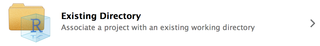
When prompted, turn your recently created “Existing Directory” into a project.

Upon completion, the name of the R Project should now be displayed in the top right corner of RStudio where it previously displayed “Project: (None)”. Once opened, .RProj files do not need to be saved. Double-clicking .Rproj files in the directory is now the best way to open RStudio. This will allow for the concurrent use of multiple R sessions and ensure the portability of file paths. Once an RStudio project is open, scripts can be opened by double-clicking individual files in the computer directory or clicking files in the “Files” tab.

Exercise 8

Let’s walk through this process and create an R project for this class.

1.12.2 Filepaths

Windows file paths are usually delimited with \. *nix file paths are usually delimited with /. Never use \ in file paths in R. \ is an escape character in R and will complicate an analysis. Fortunately, RStudio understands / in file paths regardless of operating system.

Never use setwd() in R. It is unnecessary, it makes code unreproducible across machines, and it is rude to collaborators. R Projects create a better framework for file paths. Simply treat the directory where the R Project lives as the working directory and directories inside of that directory as sub-directories.

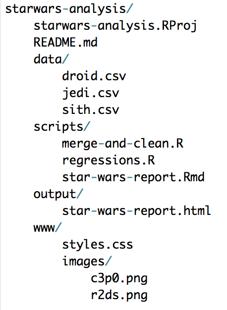
For example, say there’s a .Rproj called starwars-analysis.Rproj in a directory called starwars-analysis/. If there is a .csv in that folder called jedi.csv, the file can be loaded with read_csv("jedi.csv") instead of read_csv("H:/alena/analyses/starwars-analysis/jedi.csv"). If that file is in a sub-directory of starwars-analysis called data, it can be loaded with read_csv("data/jedi.csv"). The same concepts hold for writing data and graphics.

This simplifies code and makes it portable because all relative file paths will be identical on all computers. To share an analysis, simply send the entire directory to a collaborator or share it with GitHub.

Here’s an example directory:

1.13 Getting help

1.13.1 Googling

When Googling for R or data science help, set the search range to the last year or less to avoid out-of-date solutions and to focus on up-to-date practices. The search window can be set by clicking Tools after a Google search.

1.13.2 Stack Overflow

Stack Overflow contains numerous solutions. If a problem is particularly perplexing, it is simple to submit questions. Exercise caution when submitting questions because the Stack Overflow community has strict norms about questions and loose norms about respecting novices.

1.13.3 RStudio community

RStudio Community is a new forum for R Users. It has a smaller back catalog than Stack Overflow but users are friendlier than on Stack Overflow.

1.13.4 CRAN task views

CRAN task views contains thorough introductions to packages and techniques organized by subject matter. The Econometrics, Reproducible Research, and and Social Sciences task views are good starting places.

1.13.5 Data Science for Public Policy Slack

We’ve created a Slack workspace for this class (which will be shared across both sections) and encourage you to ask questions in Slack. In general, we ask that you try to answer questions on your own using the sources above before posting in Slack. Practicing finding and applying the relevant information to answer your questions is an important data science skill! The teaching staff will be checking the Slack to help answer questions in a reasonable time frame and we also encourage you to answer each other’s questions - it’s a great way to improve your R skills!

Questions on Slack must be asked using reproducible examples. Simply copying-and-pasting questions or answers in the Slack channel is not allowed. If you’re unsure how to share a reproducible example without sharing your answers in a public channel, you can DM the teaching staff to be safe.

1.13.6 ChatGPT:

Warning

Since there is R code on the internet, ChatGPT has been trained on R code and has the capability to answer R coding questions. Exercise extreme caution when using ChatGPT! ChatGPT saves and uses the queries you provide it. This means that asking a question about sensitive data or code could expose that data. If you decide to use ChatGPT, only ask queries of it using a reproducible example with non-sensitive data. The diamonds dataset, loaded with ggplot::diamonds(), is a great candidate.

Warning

Just like machine translators are useful for communication but can stymie the ability to learn a second language, large language models are useful for creating code but can stymie learning R.

We encourage everyone to pursue mastery of R. This means feeling the terror of the blank page and internalizing the syntax of R without the crutch of LLMs before regularly using LLMs.

ChatGPT can be a powerful tool. Some helpful tips for using ChatGPT for coding questions are:

• Provide it detailed questions
• Give it reproducible example code
• Refine queries when the initial responses are unsatisfactory

1.14 Conclusion

R is a powerful programming language that was developed initially for statistics but is now used in a variety of contexts. Key advantages to R include that it has a fantastic, custom-built IDE called RStudio and a large open source community of users that provides help and develops new packages. Like other open source programming languages, conducting data science in R supports the six principles of data analysis introduced at the start of this chapter.

Eubank, Nick. 2016. “Embrace Your Fallibility: Thoughts on Code Integrity.” https://www.nickeubank.com/wp-content/uploads/2016/06/Eubank_EmbraceYourFallibility.pdf.

Peng, Roger. 2018. “Teaching r to New Users - from Tapply to the Tidyverse.” https://simplystatistics.org/posts/2018-07-12-use-r-keynote-2018/.

Rodrigues, Bruno. 2022. Modern R with the tidyverse. https://modern-rstats.eu.

Wickham, Hadley. n.d. The tidyverse style guide. https://style.tidyverse.org/index.html.

Wickham, Hadley, Mine Çetinkaya-Rundel, and Garrett Grolemund. 2023. R for Data Science: Import, Tidy, Transform, Visualie, and Model Data. 2nd edition. Sebastopol, CA: O’Reilly.

Wickham, Hadley, and Garrett Grolemund. 2017. R for Data Science: Import, Tidy, Transform, Visualize, and Model Data. 1st ed. Paperback; O’Reilly Media. http://r4ds.had.co.nz/.

---

1. (Eubank 2016) influenced our thinking on this issue and provides proactive steps for writing high-quality code using defensive programming.

2. Though we do not focus on the Python programming language in this course, Posit appears to be expanding its focus to Python in addition to R. This is an important development to track in the data science landscape. One key update is that, in 2023, Posit hired Wes McKinney. McKinney developed the Python pandas package which offers similar functionality to the tidyverse, a collection of R packages which we will discuss next week.