base_url <- "https://www2.census.gov/programs-surveys/demo/datasets/hhp/"
week_url <- "2021/wk40/HPS_Week40_PUF_CSV.zip"

pulse_url <- paste0(base_url, week_url)

# creates data directory in working directory
# gives warning if directory already exists
dir.create("data")

# For Mac, *.nix systems:
download.file(
  pulse_url,
  destfile = "data/pulse40.zip"
)

# For Windows systems, you need to add the mode = "wb"
# argument to prevent an invalid zip file
download.file(
  pulse_url,
  destfile = "data/pulse40.zip",
  mode = "wb"
)5 Exploratory Data Analysis
Abstract
This chapter introduces exploratory data analysis (EDA), an essential process for data scientists and researchers to use to understand their data.

5.1 Reading in Data
We’ve already covered reading in csv files using the read_csv() function from the readr package, but you may also need to read in data that is stored in a number of other common file formats:
5.1.1 Excel Spreadsheets
We introduced readxl in Section 3.3.2. As a reminder, it is not a core tidyverse package, so it needs to be explicitly loaded in each R session.
Many excel files can be read with the simple syntax data <- read_excel(path = "relative/file/path/to/data"). In cases where the Excel spreadsheet contains multiple sheets, you can use the sheet argument to specify the sheet to read as a string (the name of the sheet) or an integer (the position of the sheet). You can also read only components of a sheet using Excel-style cell-ranges (ex: A3:L44).
5.1.2 STATA, SAS, and SPSS files
haven is a tidyverse package for reading data from SAS (read_sas()), STATA (read_dta()), and SPSS (read_sav()) files. Like the readxl package, it is not a core tidyverse package and also needs to be explicitly loaded in each R session.
Note that the haven package can only read and write STATA .dta files through version 15 of STATA. For files created in more recent versions of STATA, the readstat13 package’s read.dta13 file can be used.
5.1.3 Zip Files
You may also want to read in data that is saved in a zip file. In order to do this, you can use the unzip() function to unzip the files using the following syntax: unzip(zipfile = "path/to/zip/file", exdir = "path/to/directory/for/unzipped/files").
Often times, you may want to read in a zip file from a website into R. In order to do this, you will need to first download the zip file to your computer using the download.file() function, unzip the file using unzip() and then read in the data using the appropriate function for the given file type.
To download the week 40 public use file data for the Census Household Pulse Survey, run the following code:
5.2 Column Names
As discussed earlier in the course, dataframe columns - like other objects - should be given names that are “concise and meaningful”. Generally column names should be nouns and only use lowercase letters, numbers, and underscores _ (this is referred to as snake case). Columns should not begin with numbers. You should not include white space in column names (e.g “Birth Month” = bad, “birth_month” = good). It is also best practice for column names to be singular (use “birth_month” instead of “birth_months”).
The janitor package is a package that contains a number of useful functions to clean data in accordance with the tidyverse principles. One such function is the clean_names() function, which converts column names to snake case according to the tidyverse type guide (along with some other useful cleaning functions outlined in the link above). The clean_names() function works well with the |> operator.
As discussed in the introduction to the tidyverse, you can also directly rename columns using the rename() function from the dplyr package as follows: rename(data, new_col = old_col).
5.3 Data Overview
Once you’ve imported your data, a common first step is to get a very high-level summary of your data.
As introduced in the introduction to the tidyverse, the glimpse() function provides a quick view of your data, printing the type and first several values of each column in the dataset to the console.
Rows: 19,537
Columns: 13
$ name                         <chr> "Amy", "Amy", "Amy", "Amy", "Amy", "Amy",…
$ year                         <dbl> 1975, 1975, 1975, 1975, 1975, 1975, 1975,…
$ month                        <dbl> 6, 6, 6, 6, 6, 6, 6, 6, 6, 6, 6, 6, 6, 6,…
$ day                          <int> 27, 27, 27, 27, 28, 28, 28, 28, 29, 29, 2…
$ hour                         <dbl> 0, 6, 12, 18, 0, 6, 12, 18, 0, 6, 12, 18,…
$ lat                          <dbl> 27.5, 28.5, 29.5, 30.5, 31.5, 32.4, 33.3,…
$ long                         <dbl> -79.0, -79.0, -79.0, -79.0, -78.8, -78.7,…
$ status                       <fct> tropical depression, tropical depression,…
$ category                     <dbl> NA, NA, NA, NA, NA, NA, NA, NA, NA, NA, N…
$ wind                         <int> 25, 25, 25, 25, 25, 25, 25, 30, 35, 40, 4…
$ pressure                     <int> 1013, 1013, 1013, 1013, 1012, 1012, 1011,…
$ tropicalstorm_force_diameter <int> NA, NA, NA, NA, NA, NA, NA, NA, NA, NA, N…
$ hurricane_force_diameter     <int> NA, NA, NA, NA, NA, NA, NA, NA, NA, NA, N…
The summary() function enables you to quickly understand the distribution of a numeric or categorical variable. For a numeric variable, summary() will return the minimum, first quartile, median, mean, third quartile, and max values. For a categorical (or factor) variable, summary() will return the number of observations in each category. If you pass a dataframe to summary() it will summarize every column in the dataframe. You can also call summary on a single variable as shown below:
The str() function compactly displays the internal structure of any R object. If you pass a dataframe to str it will print the column type and first several values for each column in the dataframe, similar to the glimpse() function.
Getting a high-level overview of the data can help you identify what questions you need to ask of your data during the exploratory data analysis process. The rest of this lecture will outline several questions that you should always ask when exploring your data - though this list is not exhaustive and will be informed by your specific data and analysis!
5.4 Are my columns the right types?
We’ll read in the population-weighted centroids for the District of Columbia exported from the Missouri Census Data Center’s geocorr2014 tool.
Rows: 180 Columns: 7
── Column specification ────────────────────────────────────────────────────────
Delimiter: ","
chr (7): county, tract, cntyname, intptlon, intptlat, pop10, afact

ℹ Use `spec()` to retrieve the full column specification for this data.
ℹ Specify the column types or set `show_col_types = FALSE` to quiet this message.Rows: 180
Columns: 7
$ county <chr> "County code", "11001", "11001", "11001", "11001", "11001", "…
$ tract <chr> "Tract", "0001.00", "0002.01", "0002.02", "0003.00", "0004.00…
$ cntyname <chr> "County name", "District of Columbia DC", "District of Columb…
$ intptlon <chr> "Wtd centroid W longitude, degrees", "-77.058857", "-77.07521…
$ intptlat <chr> "Wtd centroid latitude, degrees", "38.909434", "38.909223", "…
$ pop10 <chr> "Total population (2010)", "4890", "3916", "5425", "6233", "1…
$ afact <chr> "tract to tract allocation factor", "1", "1", "1", "1", "1", …We see that all of the columns have been read in as character vectors because the second line of the csv file has a character description of each column. By default, read_csv uses the first 1,000 rows of data to infer the column types of a file. We can avoid this by skipping the first two lines of the csv file and manually setting the column names.
Rows: 179 Columns: 7
── Column specification ────────────────────────────────────────────────────────
Delimiter: ","
chr (2): tract, cntyname
dbl (5): county, intptlon, intptlat, pop10, afact

ℹ Use `spec()` to retrieve the full column specification for this data.
ℹ Specify the column types or set `show_col_types = FALSE` to quiet this message.Rows: 179
Columns: 7
$ county <dbl> 11001, 11001, 11001, 11001, 11001, 11001, 11001, 11001, 11001…
$ tract <chr> "0001.00", "0002.01", "0002.02", "0003.00", "0004.00", "0005.…
$ cntyname <chr> "District of Columbia DC", "District of Columbia DC", "Distri…
$ intptlon <dbl> -77.05886, -77.07522, -77.06813, -77.07583, -77.06670, -77.05…
$ intptlat <dbl> 38.90943, 38.90922, 38.90803, 38.91848, 38.92316, 38.92551, 3…
$ pop10 <dbl> 4890, 3916, 5425, 6233, 1455, 3376, 3189, 4539, 4620, 3364, 6…
$ afact <dbl> 1, 1, 1, 1, 1, 1, 1, 1, 1, 1, 1, 1, 1, 1, 1, 1, 1, 1, 1, 1, 1…You can convert column types by using the as.* set of functions. For example, we could convert the county column to a character vector as follows: mutate(dc_centroids, county = as.character(county)). We can also set the column types when reading in the data with read_csv() using the col_types argument. For example:
Rows: 179
Columns: 7
$ county   <chr> "11001", "11001", "11001", "11001", "11001", "11001", "11001"…
$ tract    <chr> "0001.00", "0002.01", "0002.02", "0003.00", "0004.00", "0005.…
$ cntyname <chr> "District of Columbia DC", "District of Columbia DC", "Distri…
$ intptlon <dbl> -77.05886, -77.07522, -77.06813, -77.07583, -77.06670, -77.05…
$ intptlat <dbl> 38.90943, 38.90922, 38.90803, 38.91848, 38.92316, 38.92551, 3…
$ pop10    <dbl> 4890, 3916, 5425, 6233, 1455, 3376, 3189, 4539, 4620, 3364, 6…
$ afact    <dbl> 1, 1, 1, 1, 1, 1, 1, 1, 1, 1, 1, 1, 1, 1, 1, 1, 1, 1, 1, 1, 1…
As you remember from week 1, a vector in R can only contain one data type. If R does not know how to convert a value in the vector to the given type, it may introduce NA values by coercion. For example:
5.4.1 String manipulation with stringr
Before converting column types, it is critical to clean the column values to ensure that NA values aren’t accidentally introduced by coercion. We can use the stringr package introduced in Section 3.5.1 to clean character data. A few reminders:
- This package is part of the core tidyverse and is automatically loaded with
library(tidyverse). - The stringr cheat sheet offers a great guide to the
stringrfunctions.
To demonstrate some of the stringr functions, let’s create a state column with the two digit state FIPS code for DC and a geoid column in the dc_centroid dataframe which contains the 11-digit census tract FIPS code, which can be useful for joining this dataframe with other dataframes that commonly use the FIPS code as a unique identifier. We will need to first remove the period from the tract column and then concatenate the county and tract columns into a geoid column. We can do that using stringr as follows:
Note
Note that the str_replace() function uses regular expressions to match the pattern that gets replaced. Regular expressions is a concise and flexible tool for describing patterns in strings - but it’s syntax can be complex and not particularly intuitive. This vignette provides a useful introduction to regular expressions, and when in doubt - there are plentiful Stack Overflow posts to help when you search your specific case. ChatGPT is often effective at writing regular expressions, but recall our warnings about using ChatGPT in Chapter 1.
5.4.2 Date manipulation with lubridate
The lubridate package, which we introduced in Section 3.5.3, makes it much easier to work with dates and times in R. As a reminder, lubridate is part of the tidyverse, but it is not a core tidyverse package. It must be explicitly loaded in each session with library(lubridate).
We’ll use a dataset on political violence and protest events across the continent of Africa in 2022 from the Armed Conflict Location & Event Data Project (ACLED) to illustrate the power of lubridate. The lubridate package allows users to easily and quickly parse date-time variables in a range of different formats. For example, the ymd() function takes a date variable in year-month-day format (e.g. 2022-01-31) and converts it to a date-time format. The different formats are outlined in the lubridate documentation.
Rows: 22101 Columns: 29
── Column specification ────────────────────────────────────────────────────────
Delimiter: ","
chr  (15): EVENT_ID_CNTY, EVENT_TYPE, SUB_EVENT_TYPE, ACTOR1, ASSOC_ACTOR_1,...
dbl  (12): ISO, EVENT_ID_NO_CNTY, YEAR, TIME_PRECISION, INTER1, INTER2, INTE...
lgl   (1): ADMIN3
dttm  (1): EVENT_DATE

ℹ Use `spec()` to retrieve the full column specification for this data.
ℹ Specify the column types or set `show_col_types = FALSE` to quiet this message.
Creating datetime columns enables the use of a number of different operations, such as filtering based on date:
# A tibble: 6,859 × 5
   event_date region          country event_type             sub_event_type
   <date>     <chr>           <chr>   <chr>                  <chr>
 1 2022-06-04 Northern Africa Algeria Protests               Peaceful protest
 2 2022-06-05 Northern Africa Algeria Protests               Peaceful protest
 3 2022-06-05 Northern Africa Algeria Protests               Peaceful protest
 4 2022-06-08 Northern Africa Algeria Protests               Peaceful protest
 5 2022-06-09 Northern Africa Algeria Protests               Peaceful protest
 6 2022-06-09 Northern Africa Algeria Protests               Peaceful protest
 7 2022-06-11 Northern Africa Algeria Protests               Peaceful protest
 8 2022-06-15 Northern Africa Algeria Strategic developments Looting/property d…
 9 2022-06-18 Northern Africa Algeria Protests               Protest with inter…
10 2022-06-19 Northern Africa Algeria Protests               Peaceful protest
# ℹ 6,849 more rows
Or calculating durations:
# A tibble: 22,101 × 6
   event_date region          country event_type sub_event_type   days_into_2022
   <date>     <chr>           <chr>   <chr>      <chr>            <drtn>
 1 2022-01-03 Northern Africa Algeria Protests   Peaceful protest 2 days
 2 2022-01-03 Northern Africa Algeria Protests   Peaceful protest 2 days
 3 2022-01-04 Northern Africa Algeria Protests   Peaceful protest 3 days
 4 2022-01-05 Northern Africa Algeria Protests   Peaceful protest 4 days
 5 2022-01-05 Northern Africa Algeria Protests   Peaceful protest 4 days
 6 2022-01-05 Northern Africa Algeria Protests   Peaceful protest 4 days
 7 2022-01-05 Northern Africa Algeria Protests   Peaceful protest 4 days
 8 2022-01-05 Northern Africa Algeria Protests   Peaceful protest 4 days
 9 2022-01-06 Northern Africa Algeria Protests   Peaceful protest 5 days
10 2022-01-06 Northern Africa Algeria Protests   Peaceful protest 5 days
# ℹ 22,091 more rows
Or extracting components of dates:
# A tibble: 22,101 × 6
event_date region country event_type sub_event_type event_month
<date> <chr> <chr> <chr> <chr> <dbl>
1 2022-01-03 Northern Africa Algeria Protests Peaceful protest 1
2 2022-01-03 Northern Africa Algeria Protests Peaceful protest 1
3 2022-01-04 Northern Africa Algeria Protests Peaceful protest 1
4 2022-01-05 Northern Africa Algeria Protests Peaceful protest 1
5 2022-01-05 Northern Africa Algeria Protests Peaceful protest 1
6 2022-01-05 Northern Africa Algeria Protests Peaceful protest 1
7 2022-01-05 Northern Africa Algeria Protests Peaceful protest 1
8 2022-01-05 Northern Africa Algeria Protests Peaceful protest 1
9 2022-01-06 Northern Africa Algeria Protests Peaceful protest 1
10 2022-01-06 Northern Africa Algeria Protests Peaceful protest 1
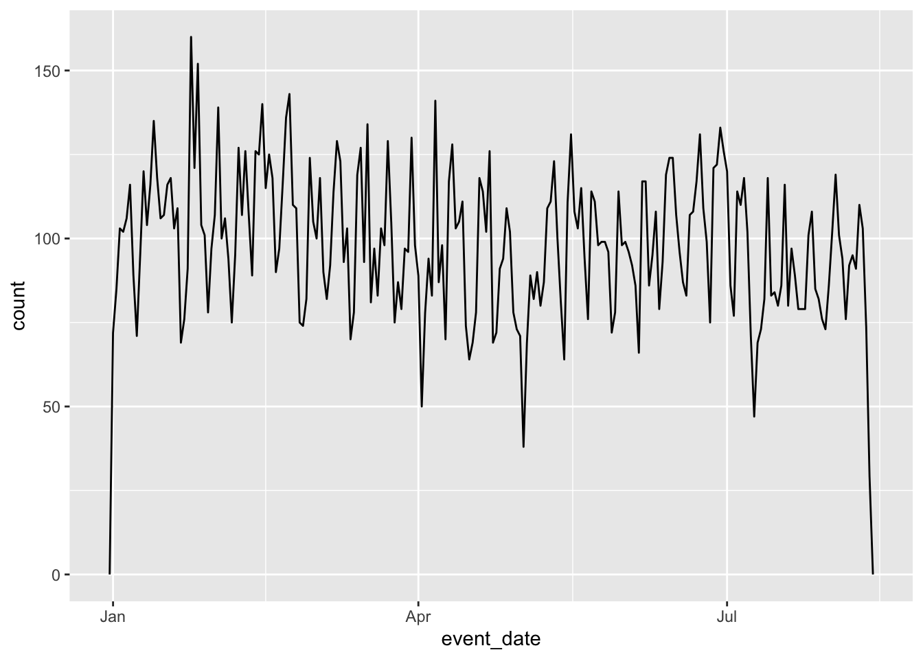
# ℹ 22,091 more rowsDatetimes can also much more easily be plotted using ggplot2. For example, it is easy to visualize the distribution of events across the year:
For more information on lubridate, see the lubridate cheat sheet.
5.4.3 Categorical and Factor Variables
Categorical variables can be stored as characters in R. The case_when() function makes it very easy to create categorical variables based on other columns. For example:
Factors are a data type specifically made to work with categorical variables. The forcats library in the core tidyverse is made to work with factors. Factors are particularly valuable if the values have a ordering that is not alphanumeric.
[1] "Apr" "Dec" "Jan" "Mar"[1] Jan Mar Apr Dec
Levels: Jan Feb Mar Apr May Jun Jul Aug Sep Oct Nov DecFactors are also valuable if you want to show all possible values of the categorical variable, even when they have no observations.
5.5 Is there missing data?
Before you work with any dataset, you should understand how missing values are encoded. The best place to find this information is the data dictionary - which you should always read before working with any new dataset!
This is particularly important because while R automatically recognizes standard missing values as NA, it doesn’t recognize non-standard encodings like numbers representing missing values, “missing”, “na”, “N/A”, etc.
Non-standard missing values should be converted to NA before conducting analysis. One way of doing this is with mutate and the if_else or case_when functions.
Once you have converted all missing value encodings to NA, the next question you need to ask is how you want to handle missing values in your analysis. The right approach will depend on what the missing value represents and the goals of your analysis.
Leave as NA: This can be the best choice when the missing value truly represents a case when the true value is unknown. You will need to handle NAs by setting
na.rm = TRUEin functions or filtering usingis.na(). One drawback of this approach is that if the values aren’t missing at random (e.g. smokers may be less likely to answer survey questions about smoking habits), your results may be biased. Additionally, this can cause you to lose observations and reduce power of analyses.Replace with 0: This can be the best choice if a missing value represents a count of zero for a given entity. For example, a dataset on the number of Housing Choice Voucher tenants by zip code and quarter may have a value of NA if there were no HCV tenants in the given zip code and quarter.
Impute missing data: Another approach is imputing the missing data with a reasonable value. There are a number of different imputation approaches:
- Mean/median/mode imputation: Fills the missing values with the column mean or median. This approach is very easy to implement, but can artifically reduce variance in your data and be sensitive to outliers in the case of mean imputation.
- Predictive imputation: Fills the missing values with a predicted value based on a model that has been fit to the data or calculated probabilities based on other columns in the data. This is a more complex approach but is likely more accurate (for example, it can take into account variable correlation).
These alternatives are discussed in more detail in a later chapter covering data imputation.
The replace_na() function in dplyr is very useful for replacing NA values in one or more columns.
# A tibble: 3 × 2
      x y
  <dbl> <chr>
1     1 a
2     2 <NA>
3     0 b
# A tibble: 3 × 2
x y
<dbl> <chr>
1 1 a
2 2 unknown
3 0 b # A tibble: 3 × 2
x y
<dbl> <chr>
1 1 a
2 2 <NA>
3 1.5 b 5.6 Do I have outliers or unexpected values?
5.6.1 Identifying Outliers/Unexpected Values
Using R to examine the distribution of your data is one way to identify outliers or unexpected values. For example, we can examine the distribution of the bodywt variable in the msleep dataset both by examining the mathematical distribution using the summary() function and visually using ggplot.
    Min.  1st Qu.   Median     Mean  3rd Qu.     Max.
0.005 0.174 1.670 166.136 41.750 6654.000 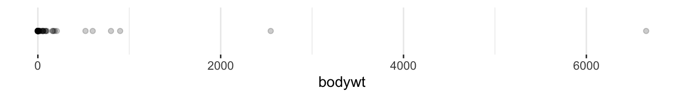
5.6.2 Unit Tests
Writing tests in R is a great way to test that your data does not have unexpected/incorrect values. These tests can also be used to catch mistakes that can be introduced by errors in the data cleaning process. There are a number of R packages that have tools for writing tests, including:
verification [age < 120] failed! (1 failure)

    verb redux_fn predicate column index value
1 verify       NA age < 120     NA     2    NA
Error: assertr stopped executionCritically, adding the test caused the code to return an error before calculating the mean of the age variable. This is a feature, not a bug! It can prevent you from introducing errors into your analyses. Moreover, by writing a set of tests in your analysis code, you can run the same checks every time you perform the analysis which can help you catch errors caused by changes in the input data.
5.6.3 Handling Outliers/Unexpected Values
When you identify outliers or unexpected values, you will have to decide how you want to handle those values in your data. The proper way to handle those values will depend on the reason for the outlier value and the objectives of your analysis.
- If the outlier is caused by data errors, such as an implausible age or population value, you can replace the outlier values with
NAusingmutateandif_elseorcase_whenas described above. - If the outlier represents a different population than the one you are studying - e.g. the different consumption behaviors of individual consumers versus wholesale business orders - you can remove it from the data.
- You can transform the data, such as taking the natural log to reduce the variation caused by outliers.
- You can select a different analysis method that is less sensitive to outliers, such as using the median rather than the mean to measure central tendency.
5.7 Data Quality Assurance
Data quality assurance is the foundation of high quality analysis. Four key questions that you should always ask when considering using a dataset for analysis are:
- Does the data suit the research question? Examine the data quality (missingness, accuracy) of key columns, the number of observations in subgroups of interest, etc.
- Does the data accurately represent the population of interest? Think about the data generation process (e.g. using 311 calls or Uber ride data to measure potholes) - are any populations likely to be over or underrepresented? Use tools like Urban’s Spatial Equity Data Tool to test data for unrepresentativeness.
- Is the data gathering reproducible? Wherever possible, eliminate manual steps to gather or process the data. This includes using reproducible processes for data ingest such as APIs or reading data directly from the website rather than manually downloading files. All edits to the data should be made programmatically (e.g. skipping rows when reading data rather than deleting extraneous rows manually). Document the source of the data including the URL, the date of the access, and specific metadata about the vintage.
- How can you verify that you are accessing and using the data correctly? This may include writing tests to ensure that raw and calculated data values are plausible, comparing summary statistics against those provided in the data documentation (if applicable), published tables/statistics from the data provider, or published tables/statistics from a trusted third party.
5.8 Conclusion
This chapter outlined EDA in great detail. Some key reminders are: - R and the tidyverse have great packages for reading in data (readr for csv files, readxl for Excel files, haven for STATA, SAS, and SPSS files).
janitor::clean_names()is a great way to get your column name structure to “snake case”.glimpse()is an easy way to get summary statistics on your columns.stringrandlubridatecan help you handle string and date manipulation, respectively.- There a many good options for handling missing data. Be thoughtful!
- Unit tests are a good way to ensure your data is in an expected format.