25  Text Modeling

Abstract

In this chapter, we introduce fundamental ideas for text modeling.

25.1 Background

25.1.1 Document-Term Matrix

There exist useful alternative formats to tidytext for storing text information. Different applications use different formats.

Document-Term Matrix

A matrix where rows are documents, columns are words, and cells are counts. A document-term matrix is typically sparse.

One-row-per document

A data frame with a column where each cell is the entire text for a document. This is useful for predictive modeling.

Example 01

library(tidyverse)

── Attaching core tidyverse packages ──────────────────────── tidyverse 2.0.0 ──
✔ dplyr     1.1.4     ✔ readr     2.1.5
✔ forcats   1.0.0     ✔ stringr   1.5.1
✔ ggplot2   3.5.1     ✔ tibble    3.2.1
✔ lubridate 1.9.3     ✔ tidyr     1.3.1
✔ purrr     1.0.2     
── Conflicts ────────────────────────────────────────── tidyverse_conflicts() ──
✖ dplyr::filter() masks stats::filter()
✖ dplyr::lag()    masks stats::lag()
ℹ Use the conflicted package (<http://conflicted.r-lib.org/>) to force all conflicts to become errors

library(tidytext)

theme_set(theme_minimal())

example_doc <- 
  tribble(
    ~document, ~word, ~n,
    "a", "apple", 3,
    "a", "orange", 2, 
    "a", "banana", 1,
    "b", "apple", 2, 
    "b", "banana", 3
  )

document_term_matrix <- example_doc |>
  cast_dtm(document = document, term = word, value = n)

# document term matrices are large and typically print like this
document_term_matrix

<<DocumentTermMatrix (documents: 2, terms: 3)>>
Non-/sparse entries: 5/1
Sparsity           : 17%
Maximal term length: 6
Weighting          : term frequency (tf)

# here we can see the actual matrix
as.matrix(document_term_matrix)

    Terms
Docs apple orange banana
   a     3      2      1
   b     2      0      3

25.1.2 library(broom)

library(broom) contains three functions for tidying up the output of models in R. Most models work with library(broom) including lm(), glm(), and kmeans().

• glance() Returns one row per model.
• tidy() Returns one row per model component (i.e. regression coefficient or cluster).
• augment() Returns one row per observation in the model data set.

25.1.3 Example 02

library(broom)

Warning: package 'broom' was built under R version 4.3.3

cars_lm <- lm(dist ~ speed, data = cars)

# one row for the model
glance(cars_lm)

# A tibble: 1 × 12
  r.squared adj.r.squared sigma statistic  p.value    df logLik   AIC   BIC
      <dbl>         <dbl> <dbl>     <dbl>    <dbl> <dbl>  <dbl> <dbl> <dbl>
1     0.651         0.644  15.4      89.6 1.49e-12     1  -207.  419.  425.
# ℹ 3 more variables: deviance <dbl>, df.residual <int>, nobs <int>

# one row per coefficient
tidy(cars_lm)

# A tibble: 2 × 5
  term        estimate std.error statistic  p.value
  <chr>          <dbl>     <dbl>     <dbl>    <dbl>
1 (Intercept)   -17.6      6.76      -2.60 1.23e- 2
2 speed           3.93     0.416      9.46 1.49e-12

# one row per observation in the modeling data
augment(cars_lm)

# A tibble: 50 × 8
    dist speed .fitted .resid   .hat .sigma  .cooksd .std.resid
   <dbl> <dbl>   <dbl>  <dbl>  <dbl>  <dbl>    <dbl>      <dbl>
 1     2     4   -1.85   3.85 0.115    15.5 0.00459       0.266
 2    10     4   -1.85  11.8  0.115    15.4 0.0435        0.819
 3     4     7    9.95  -5.95 0.0715   15.5 0.00620      -0.401
 4    22     7    9.95  12.1  0.0715   15.4 0.0255        0.813
 5    16     8   13.9    2.12 0.0600   15.5 0.000645      0.142
 6    10     9   17.8   -7.81 0.0499   15.5 0.00713      -0.521
 7    18    10   21.7   -3.74 0.0413   15.5 0.00133      -0.249
 8    26    10   21.7    4.26 0.0413   15.5 0.00172       0.283
 9    34    10   21.7   12.3  0.0413   15.4 0.0143        0.814
10    17    11   25.7   -8.68 0.0341   15.5 0.00582      -0.574
# ℹ 40 more rows

25.2 Document Grouping/Topic Modeling

The algorithmic grouping or clustering of documents using features extracted from the documents. This includes unsupervised classification of documents into meaningful groups.

Topic modeling

The unsupervised clustering, or grouping, of text documents based on their content.

• Alena Stern used Latent Dirichlet Allocation (LDA) to sort 110,063 public records requests into 60 topics (blog)
• Pew Research used unsupervised and semi-supervised methods to create topic models of open-ended text responses about where Americans find meaning in their lives. (blog)

Leveraging what we already know, we can use K-means clustering on a term-document matrix to cluster documents. This approach has two shortcomings and one advantage.

1. It takes a lot of work to summarize documents that are grouped with K-means clustering.
2. K-means clustering creates hard assignments. Each observation belongs to exactly one cluster.
3. K-means clustering uses Euclidean distance, which is relatively simple when working with text

Soft assignment

Observations are assigned to each cluster or group with probabilities or weights. For example, observation 1 belongs to Group A with 0.9 probability and Group B with 0.1 probability.

We will focus on a topic modeling algorithm called Latent Dirichlet Allocation (LDA). Non-negative matrix factorization is a different popular algorithm that we will not discuss.

Latent Dirichlet Allocation (LDA)

A probabilistic topic model where each document is a mixture of topics and each topic is a mixture of words.

25.2.1 LDA as a generative model

LDA is a generative model. The model describes how the documents in a corpus were created. LDA relies on the bag-of-words assumption.

Bag-of-words assumption

Disregard the grammar and order of words.

According to the model, any time a document is created:

1. Choose the length of the document, \(N\), from a probability distribution
2. Randomly choose topic probabilities for a document
3. For each word in the document
   1. Randomly choose a topic
   2. Randomly choose a word conditioned on the topic from a.

25.2.2 Example 03

Let’s demonstrate generating a document using this model. First, let’s define two topics. topic1 is about the economy and topic2 is about sports. Note that “contract” and “union” are in both topics:

topic1 <- c(
  "inflation", 
  "unemployment", 
  "labor", 
  "force", 
  "exchange",
  "rate",
  "dollar",
  "bank",
  "employer",
  "gdp",
  "federal",
  "reserve",
  "return",
  "nasdaq",
  "startup",
  "business",
  "insurance",
  "labor",
  "union",
  "contract"
)

topic2 <- c(
  "basketball", 
  "basket", 
  "playoff", 
  "goal", 
  "referee",
  "win",
  "loss",
  "score",
  "soccer",
  "polo",
  "run",
  "champion",
  "trophy",
  "contract",
  "union",
  "arena",
  "stadium",
  "concession",
  "court",
  "lights"
)

topics <- list(
  topic1,
  topic2
)

Next, randomly sample a document length. In this case, we will use the Poisson distribution, which returns non-negative integers. We use _i to note that this is for the \(i^{th}\) document.

set.seed(42)

document_length_i <- rpois(n = 1, lambda = 10)

document_length_i

[1] 14

Each document will have a document-specific topic probability distribution. We use the Dirichlet distribution to generate this vector of probabilities. The Dirichlet distribution is a multivariate beta distribution. The beta distribution returns random draws between 0 and 1 and is related to the standard uniform distribution.

topic_distribution_i <- MCMCpack::rdirichlet(n = 1, alpha = c(0.5, 0.5)) |>
  as.numeric()

topic_distribution_i

[1] 0.1311192 0.8688808

Using the document-specific topic distribution, we randomly assign a topic for each of the 14 words in our document.

topic_j <- sample(
  x = 1:2, 
  size = document_length_i, 
  prob = topic_distribution_i, 
  replace = TRUE
)

topic_j

 [1] 2 2 2 2 1 2 2 1 1 2 2 2 1 2

Finally, we sample each word from the sampled topic.

document_i <- map_chr(
  .x = topic_j,
  .f = ~sample(x = topics[[.x]], size = 1)
)

document_i

 [1] "soccer"     "goal"       "referee"    "trophy"     "exchange"  
 [6] "lights"     "basket"     "bank"       "labor"      "basketball"
[11] "polo"       "run"        "startup"    "score"     

We have now generated a document that is a mixture of the two topics. It’s more sports than economics, but contains both topics.

The topics are also mixtures of words. “Basketball” only shows up in the sports topic but “union” and “contract” are in both topics. When used in practice, LDA generally involves more words, more topics, and more documents.

25.2.3 LDA and inference

LDA is based on this data generation process, but we don’t know the document-specific topic distribution or the topics for the individual words. Thus, LDA is a statistical inference procedure where we try to make inferences about parameters. In other words, we are trying to reverse engineer the generative process outlined above using a corpus of documents. In practice, we don’t care about the length of the document, so we can ignore step 1.

The optimization for LDA is similar to the optimization for K-means clustering. First, every word in the corpus is randomly assigned a topic. Then, the model is optimized through a two-step process based on expectation maximization (EM), which is the same optimization algorithm used with K-means clustering:

1. Find the optimal posterior topic distribution for each document (this is \(\theta\) indirectly) assuming the prior parameters are known
2. Find the optimal prior parameters assuming the posterior topic distribution for each document is known
3. Repeat steps 1. and 2. until some topping criterion is reached

25.2.4 Example 04

Let’s consider the executive orders data set. We repeat the pre-processing from the past example but with even more domain-specific stop words. Note: this example builds heavily on Chapter 6 in Text Mining With R.

library(tidyverse)
library(tidytext)
library(SnowballC)
library(topicmodels)

Warning: package 'topicmodels' was built under R version 4.3.3

# load one-row-per-line data ----------------------------------------------
eos <- read_csv(here::here("data", "executive-orders.csv"))

Rows: 196537 Columns: 4
── Column specification ────────────────────────────────────────────────────────
Delimiter: ","
chr  (2): text, president
dbl  (1): executive_order_number
date (1): signing_date

ℹ Use `spec()` to retrieve the full column specification for this data.
ℹ Specify the column types or set `show_col_types = FALSE` to quiet this message.

eos <- filter(eos, !is.na(text))

# tokenize the text -------------------------------------------------------
tidy_eos <- eos |>
  unnest_tokens(output = word, input = text)

# create domain-specific stop words
domain_stop_words <- tribble(
  ~word, 
  "william",
  "clinton",
  "george",
  "bush", 
  "barack",
  "obama", 
  "donald",
  "trump",
  "joseph",
  "biden",
  "signature",
  "section",
  "authority",
  "vested",
  "federal",
  "president",
  "authority",
  "constitution",
  "laws",
  "united",
  "states",
  "america",
  "secretary",
  "assistant",
  "executive",
  "order",
  "sec",
  "u.s.c",
  "pursuant",
  "act",
  "law"
) |>
  mutate(lexicon = "custom")

stop_words <- bind_rows(
  stop_words,
  domain_stop_words
)

# remove stop words with anti_join() and the stop_words tibble
tidy_eos <- tidy_eos |>
  anti_join(stop_words, by = "word") 

# remove words that are entirely numbers
tidy_eos <- tidy_eos |>
  filter(!str_detect(word, pattern = "^\\d")) 

# stem words with wordStem()
tidy_eos <- tidy_eos |>
  mutate(stem = wordStem(word))

Next, we convert the tidytext executive orders into a document-term matrix with cast_dtm().

tidy_eos_count <- tidy_eos |>
  count(president, executive_order_number, stem) 

eos_dtm <- tidy_eos_count |>
  cast_dtm(document = executive_order_number, term = stem, value = n)

Once we have a document-term matrix, implementing LDA is straightforward with LDA(), which comes from library(topicmodels). We must predetermine the number of groups with k and we set the seed because the algorithm is stochastic (not deterministic).

eos_lda <- eos_dtm |>
  LDA(k = 22, control = list(seed = 20220417))

Note: I chose 22 topics using methods outlined in the appendix.

Interpreting an estimated LDA model is the tricky work. We will do this by looking at

1. Each topic as a mixture of words
2. Each document as a mixture of topics

Word topic probabilities

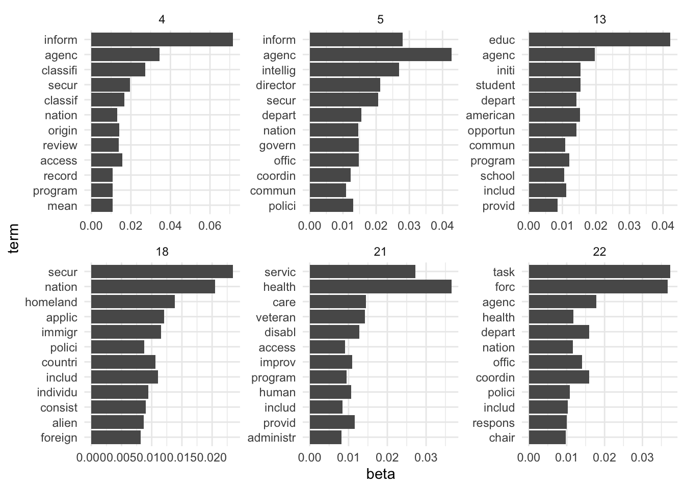
With LDA, each topic is a mixture of words. The model returns estimated parameters called \(\beta\). A \(\beta\) represents the estimated probability of a specific word being generated from a particular topic. We can extract \(\beta\) from the output of LDA() with tidy().

lda_beta <- tidy(eos_lda, matrix = "beta")

top_beta <- lda_beta |>
  group_by(topic) |>
  slice_max(beta, n = 12) |>
  ungroup() |>
  arrange(desc(beta))

top_beta

# A tibble: 264 × 3
   topic term       beta
   <int> <chr>     <dbl>
 1     2 schedul  0.0863
 2     4 inform   0.0716
 3     6 committe 0.0630
 4     6 amend    0.0540
 5     2 pai      0.0488
 6    11 contract 0.0449
 7    17 agenc    0.0441
 8     5 agenc    0.0427
 9    20 agenc    0.0426
10    13 educ     0.0422
# ℹ 254 more rows

# pick 6 random topics for visualization
random_topics <- sample(1:22, size = 6)

top_beta |>
  filter(topic %in% random_topics) |>
  mutate(term = reorder(term, beta)) |>
  ggplot(aes(x = beta, y = term)) +
  geom_col() +
  facet_wrap(~ topic, scales = "free")

Document-topic probabilities

With LDA, each document is a mixture of topics The model returns estimated parameters called \(\gamma\). A \(\gamma\) represents the estimated proportion of words from a specific document that come from a particular topic.

lda_gamma <- tidy(eos_lda, matrix = "gamma")

top_gamma <- lda_gamma |>
  group_by(topic) |>
  slice_max(gamma, n = 12) |>
  ungroup() |>
  arrange(desc(gamma))

top_gamma

# A tibble: 266 × 3
   document topic gamma
   <chr>    <int> <dbl>
 1 13086       14  1.00
 2 13262       14  1.00
 3 13292        4  1.00
 4 12958        4  1.00
 5 13693       17  1.00
 6 13123       17  1.00
 7 13780       18  1.00
 8 13951       21  1.00
 9 13178       12  1.00
10 13645       10  1.00
# ℹ 256 more rows

LDA isn’t perfect. It can result in topics that are too broad (what Patrick van Kessel calls “undercooked”) or topics that are too granular (what van Kessel calls “overcooked”).

In a related blog, van Kessel discusses using a semi-supervised algorithm called CorEx to resolve some of these challenges. With semi-supervised learning, the analyst can provide anchor terms that help the algorithm generate topics that are better cooked than with unsupervised learning.

25.3 Text Classification (supervised machine learning)

Sometimes it is useful to create a predictive model that uses text to predict a pre-determined set of labels. For example, if you have a historical corpus of labeled documents and you want to predict labels for new documents. For example, if you have a massive corpus set with a hand-labeled random sample of documents and you want to scale those labels to all documents.

Fortunately, we can use all of the library(tidymodels) tools we already learned this semester. We simply need a way to convert unstructured text into predictors, which is simple with library(textrecipes).

25.4 library(textrecipes)

library(textrecipes) augments library(recipes) with step_*() functions that are useful for supervised machine learning with text data.

• step_tokenize() Create a token variable from a character predictor.
• step_tokenfilter() Remove tokens based on rules about the frequency of tokens.
• step_tfidf() Create multiple variables with TF-IDF.
• step_ngram() Create a token variable with n-grams.
• step_stem() Stem tokens.
• step_lemma() Lemmatizes tokens with library(spacyr).
• step_stopwords() Remove stopwords.

25.4.1 Example 05

Consider the Federalist Papers data set we used in the earlier class notes. After loading the data, the data are in one-row-per-line format. This is the format that we tidied with unnest_tokens().

# A tibble: 6,089 × 3
   text                                                      paper_number author
   <chr>                                                            <int> <chr> 
 1 "THE FEDERALIST PAPERS  By Alexander Hamilton, John Jay,…            1 hamil…
 2 " 1  General Introduction  For the Independent Journal"              1 hamil…
 3 " Saturday, October 27, 1787   HAMILTON  To the People o…            1 hamil…
 4 " The subject speaks its own importance; comprehending i…            1 hamil…
 5 " It has been frequently remarked that it seems to have …            1 hamil…
 6 " If there be any truth in the remark, the crisis at whi…            1 hamil…
 7 "  This idea will add the inducements of philanthropy to…            1 hamil…
 8 " Happy will it be if our choice should be directed by a…            1 hamil…
 9 " But this is a thing more ardently to be wished than se…            1 hamil…
10 " The plan offered to our deliberations affects too many…            1 hamil…
# ℹ 6,079 more rows

Predictive modeling uses a slightly different data format than tidytext. We want each row in the data to correspond with the observations we are using for predictions. In this case, we want one row per Federalist paper.

We can use nest() and paste() to transform the data into this format.

fed_papers <- fed_papers |>
  group_by(paper_number) |>
  nest(text = text) |>
  # paste individual lines into one row per document
  mutate(text = map_chr(.x = text, ~paste(.x[[1]], collapse = " "))) |>
  ungroup() |>
  # remove white spaces
  mutate(text = str_squish(str_to_lower(text)))

fed_papers

# A tibble: 85 × 3
   paper_number author   text                                                   
          <int> <chr>    <chr>                                                  
 1            1 hamilton "the federalist papers by alexander hamilton, john jay…
 2            2 jay      "federalist no 2 concerning dangers from foreign force…
 3            3 jay      "\" publius federalist no 3 the same subject continued…
 4            4 jay      "publius federalist no 4 the same subject continued (c…
 5            5 jay      "publius federalist no 5 the same subject continued (c…
 6            6 hamilton "publius federalist no 6 concerning dangers from disse…
 7            7 hamilton "federalist no 7 the same subject continued (concernin…
 8            8 hamilton "federalist no 8 the consequences of hostilities betwe…
 9            9 hamilton "federalist no 9 the union as a safeguard against dome…
10           10 madison  "federalist no 10 the same subject continued (the unio…
# ℹ 75 more rows

Let’s prep() and bake() a recipe. We want to use recipes because most of these step_*() functions are data dependent and need to be repeated during resampling.

library(textrecipes)

Loading required package: recipes

Attaching package: 'recipes'

The following object is masked from 'package:stringr':

    fixed

The following object is masked from 'package:stats':

    step

recipe( ~ text, data = fed_papers) |>
  # tokenize the text
  step_tokenize(text) |>
  # remove stop works
  step_stopwords(text) |>
  # stem words
  step_stem(text) |>
  # remove infrequent tokens
  step_tokenfilter(text, max_tokens = 10) |>
  # perform TF-IDF
  step_tfidf(text) |>
  prep() |>
  bake(new_data = NULL)

# A tibble: 85 × 10
   tfidf_text_can tfidf_text_constitut tfidf_text_govern tfidf_text_mai
            <dbl>                <dbl>             <dbl>          <dbl>
 1         0.0381               0.127             0.108          0.133 
 2         0                    0                 0.0990         0.0444
 3         0.0235               0                 0.147          0.0446
 4         0.0678               0                 0.167          0.0804
 5         0.0189               0                 0.0533         0.0359
 6         0.0263               0.0263            0.0495         0.0375
 7         0.0320               0.0107            0.0301         0.0304
 8         0.0104               0.0519            0.0391         0.0788
 9         0.0104               0.0519            0.185          0.0492
10         0.0393               0.0295            0.157          0.149 
# ℹ 75 more rows
# ℹ 6 more variables: tfidf_text_must <dbl>, tfidf_text_nation <dbl>,
#   tfidf_text_on <dbl>, tfidf_text_peopl <dbl>, tfidf_text_power <dbl>,
#   tfidf_text_state <dbl>

25.4.2 Example 06

Let’s finish with an example using the executive orders data set. The data contain executive orders for presidents Clinton, Bush, Obama, Trump, and Biden. We will build a model that predicts the party of the president associated with each executive order. Even though we know the party, we can

1. predict the party of future executive orders
2. see which predictors are most predictive of party

First, we need to load and pre-process the data.

eos <- read_csv(here::here("data", "executive-orders.csv"))

Rows: 196537 Columns: 4
── Column specification ────────────────────────────────────────────────────────
Delimiter: ","
chr  (2): text, president
dbl  (1): executive_order_number
date (1): signing_date

ℹ Use `spec()` to retrieve the full column specification for this data.
ℹ Specify the column types or set `show_col_types = FALSE` to quiet this message.

# remove empty rows
eos <- filter(eos, !is.na(text))

# remove numbers
eos <- eos |>
  mutate(text = str_remove_all(text, "\\d")) |>
  mutate(text = str_remove_all(text, "``''")) |>
  mutate(text = str_squish(text))

# combine rows into one row per document
eos <- eos |>
  group_by(executive_order_number) |>
  nest(text = text) |>
  mutate(text = map_chr(.x = text, ~paste(.x[[1]], collapse = " "))) |>
  ungroup()

# label the party of each executive order
republicans <- c("bush", "trump")

eos_modeling <- eos |>
  mutate(
    party = if_else(
      condition = president %in% republicans, 
      true = "rep", 
      false = "dem"
    )
  ) |>
  # we can include non-text predictors but we drop predictors that would be too
  # useful (i.e. dates align with individual presidents)
  select(-president, -signing_date, -executive_order_number)

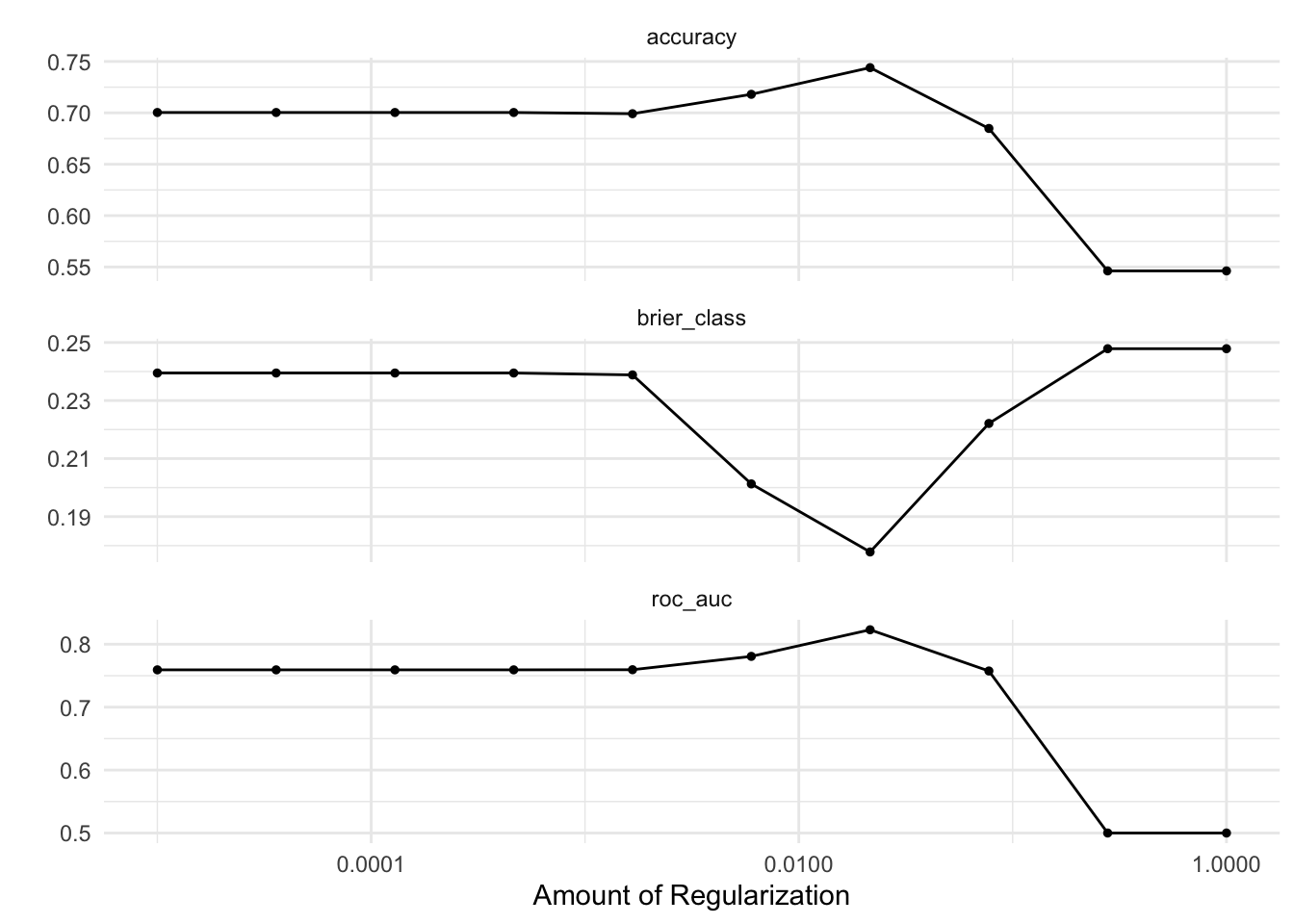
25.4.3 Logistic LASSO regression

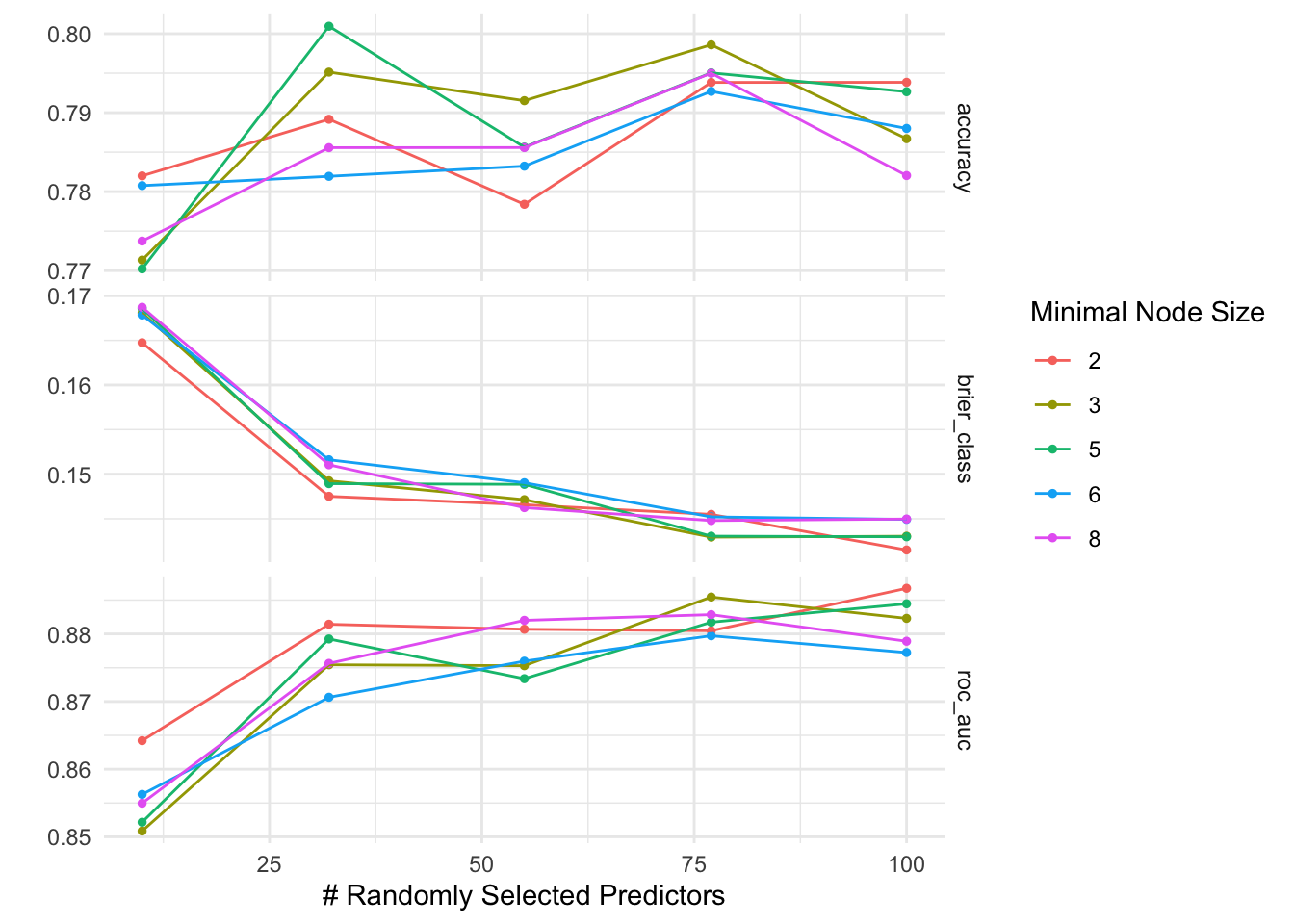
We will test a parametric (logistic LASSO regression) and a non-parametric(random forest) to predict the party using only the text of the executive orders. We will use cross-validation for model selection.

library(tidymodels)

── Attaching packages ────────────────────────────────────── tidymodels 1.2.0 ──

✔ dials        1.2.1     ✔ tune         1.2.1
✔ infer        1.0.7     ✔ workflows    1.1.4
✔ modeldata    1.4.0     ✔ workflowsets 1.1.0
✔ parsnip      1.2.1     ✔ yardstick    1.3.1
✔ rsample      1.2.1     

Warning: package 'modeldata' was built under R version 4.3.3

── Conflicts ───────────────────────────────────────── tidymodels_conflicts() ──
✖ scales::discard() masks purrr::discard()
✖ dplyr::filter()   masks stats::filter()
✖ recipes::fixed()  masks stringr::fixed()
✖ dplyr::lag()      masks stats::lag()
✖ yardstick::spec() masks readr::spec()
✖ recipes::step()   masks stats::step()
• Use tidymodels_prefer() to resolve common conflicts.

library(textrecipes)
library(vip)

Attaching package: 'vip'

The following object is masked from 'package:utils':

    vi

# create a training/testing split
set.seed(43)

eos_split <- initial_split(eos_modeling, strata = party)
eos_train <- training(eos_split)
eos_test <- testing(eos_split)

# set up cross validation
set.seed(34)
eos_folds <- vfold_cv(eos_train, strata = party)

Next, let’s create a recipe that will be used by both models.

eos_rec <-
  recipe(party ~ text, data = eos_train) |>
  step_tokenize(text) |>
  step_stopwords(text) |>
  step_stem(text) |>
  # ad hoc testing indicates that increasing max tokens makes a difference
  step_tokenfilter(text, max_tokens = 1000) |>
  step_tfidf(text) 

Create a workflow.

lasso_mod <-
  logistic_reg(penalty = tune(), mixture = 1) |>
  set_mode("classification") |>
  set_engine("glmnet")

lasso_wf <- workflow() |>
  add_recipe(eos_rec) |>
  add_model(lasso_mod)

Create a grid for hyperparameter tuning and fit the models.

lasso_grid <- grid_regular(penalty(range = c(-5, 0)), levels = 10)

lasso_cv <-
  tune_grid(
    lasso_wf,
    eos_folds,
    grid = lasso_grid
  )

Unpack the estimated models.

lasso_cv |>
  collect_metrics()

# A tibble: 30 × 7
     penalty .metric     .estimator  mean     n std_err .config              
       <dbl> <chr>       <chr>      <dbl> <int>   <dbl> <chr>                
 1 0.00001   accuracy    binary     0.700    10  0.0160 Preprocessor1_Model01
 2 0.00001   brier_class binary     0.239    10  0.0127 Preprocessor1_Model01
 3 0.00001   roc_auc     binary     0.759    10  0.0178 Preprocessor1_Model01
 4 0.0000359 accuracy    binary     0.700    10  0.0160 Preprocessor1_Model02
 5 0.0000359 brier_class binary     0.239    10  0.0127 Preprocessor1_Model02
 6 0.0000359 roc_auc     binary     0.759    10  0.0178 Preprocessor1_Model02
 7 0.000129  accuracy    binary     0.700    10  0.0160 Preprocessor1_Model03
 8 0.000129  brier_class binary     0.239    10  0.0127 Preprocessor1_Model03
 9 0.000129  roc_auc     binary     0.759    10  0.0178 Preprocessor1_Model03
10 0.000464  accuracy    binary     0.700    10  0.0160 Preprocessor1_Model04
# ℹ 20 more rows

autoplot(lasso_cv)

lasso_cv |>
  select_best(metric = "roc_auc")

# A tibble: 1 × 2
  penalty .config              
    <dbl> <chr>                
1  0.0215 Preprocessor1_Model07

Fit the best model on all of the training data and look at the coefficients.

lasso_wf <- finalize_workflow(x = lasso_wf, parameters = select_best(lasso_cv, metric = "roc_auc"))

lasso_fit <- last_fit(lasso_wf, split = eos_split)

lasso_fit |>
  extract_fit_parsnip() |>
  tidy() |>
  arrange(desc(abs(estimate))) |>
  print(n = 20)

# A tibble: 1,001 × 3
   term                estimate penalty
   <chr>                  <dbl>   <dbl>
 1 tfidf_text_bill        186.   0.0215
 2 tfidf_text_wide        -82.7  0.0215
 3 tfidf_text_avail        67.1  0.0215
 4 tfidf_text_page         65.8  0.0215
 5 tfidf_text_america'     64.6  0.0215
 6 tfidf_text_prosecut     58.2  0.0215
 7 tfidf_text_pose         56.2  0.0215
 8 tfidf_text_b            53.8  0.0215
 9 tfidf_text_earli       -53.7  0.0215
10 tfidf_text_solicit     -43.7  0.0215
11 tfidf_text_relev       -41.4  0.0215
12 tfidf_text_releas      -40.9  0.0215
13 tfidf_text_month       -33.6  0.0215
14 tfidf_text_j            33.3  0.0215
15 tfidf_text_iii          32.0  0.0215
16 tfidf_text_propos       30.9  0.0215
17 tfidf_text_on           27.0  0.0215
18 tfidf_text_deliveri     26.5  0.0215
19 tfidf_text_expertis    -25.1  0.0215
20 tfidf_text_issuanc      25.0  0.0215
# ℹ 981 more rows

25.4.4 Random forest

Create a workflow.

rf_mod <-
  rand_forest(mtry = tune(), trees = 100, min_n = tune()) |>
  set_mode("classification") |>
  set_engine("ranger", importance = "impurity")

rf_wf <- workflow() |>
  add_recipe(eos_rec) |>
  add_model(rf_mod)

Create a grid for hyperparameter tuning and fit the models.

rf_grid <- grid_regular(
  mtry(range = c(10, 100)),
  min_n(range = c(2, 8)),
  levels = 5
)

rf_cv <-
  tune_grid(
    rf_wf,
    eos_folds,
    grid = rf_grid
  )

Unpack the estimated models.

rf_cv |>
  collect_metrics()

# A tibble: 75 × 8
    mtry min_n .metric     .estimator  mean     n std_err .config              
   <int> <int> <chr>       <chr>      <dbl> <int>   <dbl> <chr>                
 1    10     2 accuracy    binary     0.782    10 0.0132  Preprocessor1_Model01
 2    10     2 brier_class binary     0.165    10 0.00604 Preprocessor1_Model01
 3    10     2 roc_auc     binary     0.864    10 0.0159  Preprocessor1_Model01
 4    32     2 accuracy    binary     0.789    10 0.0136  Preprocessor1_Model02
 5    32     2 brier_class binary     0.148    10 0.00701 Preprocessor1_Model02
 6    32     2 roc_auc     binary     0.881    10 0.0163  Preprocessor1_Model02
 7    55     2 accuracy    binary     0.778    10 0.0138  Preprocessor1_Model03
 8    55     2 brier_class binary     0.147    10 0.00677 Preprocessor1_Model03
 9    55     2 roc_auc     binary     0.881    10 0.0148  Preprocessor1_Model03
10    77     2 accuracy    binary     0.794    10 0.0153  Preprocessor1_Model04
# ℹ 65 more rows

autoplot(rf_cv)

rf_cv |>
  select_best(metric = "roc_auc")

# A tibble: 1 × 3
   mtry min_n .config              
  <int> <int> <chr>                
1   100     2 Preprocessor1_Model05

Fit the best model on all of the training data and look at variable importance.

rf_wf <- finalize_workflow(x = rf_wf, parameters = select_best(rf_cv, metric = "roc_auc"))

rf_fit <- last_fit(rf_wf, split = eos_split)

rf_fit |> 
  extract_fit_parsnip() |> 
  vip(num_features = 20)

25.4.5 Out-of-sample error rate

collect_metrics(rf_fit)

# A tibble: 3 × 4
  .metric     .estimator .estimate .config             
  <chr>       <chr>          <dbl> <chr>               
1 accuracy    binary         0.809 Preprocessor1_Model1
2 roc_auc     binary         0.877 Preprocessor1_Model1
3 brier_class binary         0.149 Preprocessor1_Model1

25.5 Resources

• Multiclass predictive modeling for #TidyTuesday NBER papers by Julia Silge
• Supervised Machine Learning for Text Analysis in R by Emil Hvitfledt and Julia Silge
• Latent Dirichlet Allocation
• Latent Dirichlet Allocation tutorial
• Computing for the Social Sciences

25.6 Appendix A

Like with cluster analysis, we need to identify a sensible number of topics for topic modeling.

Start with the application:

• Is there a policy or programmatic number that makes sense for the application?
• What have others done?
• What do subject matter experts sense is a reasonable number of topics?

There are also computational approaches to measuring the quality of the resulting topics.

This blog describes “coherence”. This resource describes a related measure called perplexity.

We can use library(ldatuning) to determine the optimal number of topics for LDA.

• library(ldatuning) page
• library(ldatuning) vignette

It is computationally expensive. FindTopicsNumber_plot() shows the measures and labels them based on if th measures should be minimized or maximized.

library(ldatuning)

results <- FindTopicsNumber(
  eos_dtm,
  topics = seq(from = 2, to = 82, by = 10),
  # note: "Griffiths2004" does not work on Mac M1 chips because of Rmpfr
  metrics = c("CaoJuan2009", "Arun2010", "Deveaud2014"),
  method = "Gibbs",
  control = list(seed = 77),
  mc.cores = 6L,
  verbose = TRUE
)

FindTopicsNumber_plot(results)
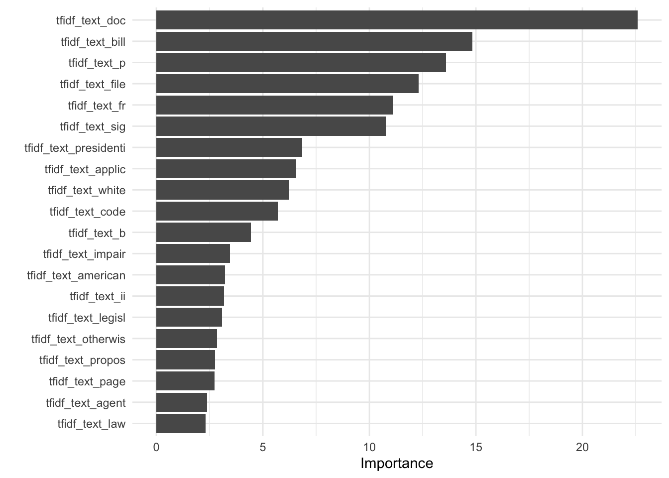