17  Predictive Modeling Motivation

Abstract

This chapter motivates predictive modeling.

17.1 Problem Structure

There are many policy applications where it is useful to make accurate predictions on “unseen” data. Unseen data means any data not used to develop a model for predictions.

The broad process of developing models to make predictions of a pre-defined variable is predictive modeling or supervised machine learning. The narrower process of developing a specific model with data is called fitting a model, learning a model, or estimating a model. The pre-defined variable the model is intended to predict is the outcome variable and the remaining variables used to predict the outcome variable are predictors.¹

In most applications we have modeling data that include the outcome of interest and implementation data that do not include the outcome of interest. Our objective is to fit, or estimate, some \(\hat{f}(\vec{x})\) using the modeling data to predict the missing outcome in the implementation data.

Figure 17.1: Modeling Data and Implementation Data for predicting the presence of lead in homes

Modeling Data

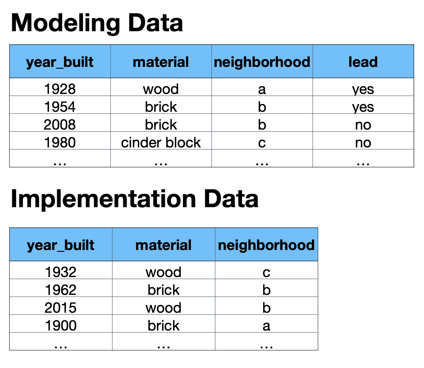
Modeling data contain the outcome variable of interest, and predictors for fitting models to predict the outcome variable of interest.

Modeling data are often historical data or high-cost data.

Implementation Data

Implementation data contain predictors for predicting the outcome of interest but don’t necessarily contain the outcome of interest.

The implementation data needs to contain all of the predictors used in the modeling data, and the implementation data can’t be too different from the modeling data.

Figure 17.2: Using modeling data to fit a model and make predctions on the implementation data

Our fitted models never perfectly predict the outcome, \(y\). Therefore, we end up with \(y = \hat{f}(\vec{x}) + \epsilon\). A major effort in predictive modeling is improving \(\hat{f}(\vec{x})\) to reduce \(\epsilon\).

17.2 Example: Marbles

17.2.1 Implementation Data

Size	Color
Small	?
Big	?
Big	?

17.2.2 Modeling Data

Size	Color
Small	Red
Small	Red
Small	Red
Small	Red
Small	Blue
Big	Red
Big	Blue
Big	Blue
Big	Blue
Big	Blue

17.2.3 Predictive Model

Challenge

How can we predict color in the implementation data?

Solution

A simple decision tree works well here! Predictive modeling! Machine learning!

• If a marble is small, then predict Red
• If a marble is big, then predict Blue

Most predictive modeling is repeating this type of learning in higher-dimensional applications where it is tougher to see the model with a glance.

17.3 Applications

Predictive modeling has many applications in public policy. Predictive models can be used to improve the allocation of scarce resources, scale survey responses or hand-labelled data sets, and forecast or nowcast.

17.3.1 Targeting Interventions

Targeting Interventions

Using predictive modeling to target the person, household, or place most in need of a policy intervention. Effective targeting can maximize the impact of a limited intervention.

17.3.2 Amplified Asking

Amplified Asking

Amplified asking (Salganik 2018) uses predictive modeling trained on a small amount of survey data from one data source and applies it to a larger data source to produce estimates at a scale or geographic granularity not possible with either data set on its own.

17.3.3 Scaled Labeling

Scaled Labeling

The process of labeling a subset of data and then using predictive models to label the full data.

This is most effective when labeling the data is time consuming or expensive.

17.3.4 Forecasting and Nowcasting

Forecasting and Nowcasting

A forecast attempts to predict the most-likely future. A nowcast attempts to predict the most-likely present in situations where information is collected and reported with a lag.

17.3.5 Imputation

Broadly, imputation is the task of using models to assign, or impute, missing values in some dataset. Broadly, imputation can be used for a variety of applications including trying to reduce the consequences of omitted variable bias, generating synthetic data to minimize disclosure risks, and data fusion. Amplified asking and scaled labeling are also examples of imputation tasks.

17.4 Case Studies

17.4.1 Preventing Lead Poisoning

Consider “Predictive Modeling for Public Health: Preventing Childhood Lead Poisoning” by Potash et al. (2015).

The authors use historical data in Chicago from home lead inspectors and observable characteristics about homes and neighborhoods to predict if homes contain lead.

• Motivation: Lead poisoning is terrible for children, but Chicago has limited lead inspectors.
• Implementation data: Observed characteristics about homes and neighborhoods in Chicago.
• Modeling data: Historical characteristics about homes and neighborhoods in Chicago and results from home lead inspections.
• Objective: Predict the probability of a home containing lead. 1. Prioritize sending inspectors to the homes of the most at-risk children before the child suffers from elevated blood lead level (BLL). 2. Create a risk score for children that can be used by parents and health providers.
• Tools: Cross validation and regularized logistic regression, linear SVC, and Random Forests.
• Results: The precision of the model was two to five times better than the baseline scenario of randomly sending inspectors. The advantage faded over time and in situations where more inspectors were available.

17.4.2 Measuring Wealth in Rwanda

Consider “Calling for Better Measurement: Estimating an Individual’s Wealth and Well-Being from Mobile Phone Transaction Records” by Blumenstock (n.d.) and “Predicting poverty and wealth from mobile phone metadata” by Blumenstock, Cadamuro, and On (2015).

• Motivation: Measuring wealth and poverty in developing nations is challenging and expensive.
• Implementation data: 2005-2009 phone metadata from about 1.5 million phone customers in Rwanda.
• Modeling data: A follow-up phone stratified survey of 856 phone customers with questions about asset ownership, home ownership, and basic welfare indicators linked to the phone metadata.
• Objective: Use the phone metadata to accurately predict variables about asset ownership, home ownership, and basic welfare indicators. One of their outcomes variables is the first principal component of asset variables.
• Tools: 5-fold cross-validation, elastic net regression and regularized logistic regression, deterministic finite automation.
• Results: The results in the first paper were poor, but follow-up work resulted in models with AUC as high as 0.88 and \(R^2\) as high as 0.46.

17.4.3 Collecting Land-Use Reform Data

Consider “How Urban Piloted Data Science Techniques to Collect Land-Use Reform Data” by Zheng (2020).

• Motivation: Land-use reform and zoning are poorly understood at the national level. The Urban Institute set out to create a data set from newspaper articles that reflects land-use reforms.
• Implementation data: About 76,000 newspaper articles
• Modeling data: 568 hand-labelled newspaper articles
• Objective: Label the nature of zoning reforms on roughly 76,000 newspaper articles.
• Tools: Hand coding, natural language processing, cross-validation, and random forests
• Results: The results were not accurate enough to treat as a data set but could be used to target subsequent hand coding and investigation.

17.4.4 Google Flu Trends

Consider the high-profile Google Flu Trends model by Ginsberg et al. (2009).

• Motivation: The CDC tracks flu-like illnesses and releases data on about a two-week lag. Understanding flu-like illnesses on a one-day lag can improve public health responses.
• Implementation data: Real-time counts of Google search queries.
• Modeling data: 2003-2008 CDC data about flu-like illnesses and counts for 50 million of the most common Google search queries in each state.
• Objective: Predict regional-level flu outbreaks on a one-day lag using Google searches to make predictions.
• Tools: Logistic regression and the top 45 influenza related illness query terms.
• Results: The in-sample results were very promising. Unfortunately, the model performed poorly when implemented. Google implemented Google Flu Trends but later discontinued the model. The two major issues were:
  1. Drift: The model decayed over time because of changes to search
  2. Algorithmic confounding: The model overestimated the 2009 flu season because of fear-induced search traffic during the Swine flu outbreak

Exercise 1

1. What other policy applications do you know for making accurate predictions on unseen data?

Blumenstock, Joshua. n.d. “Calling for Better Measurement: Estimating an Individual’s Wealth and Well-Being from Mobile Phone Transaction Records.” Center for Effective Global Action. https://escholarship.org/uc/item/8zs63942.

Blumenstock, Joshua, Gabriel Cadamuro, and Robert On. 2015. “Predicting Poverty and Wealth from Mobile Phone Metadata.” Science 350 (6264): 1073–76. https://doi.org/10.1126/science.aac4420.

Ginsberg, Jeremy, Matthew H. Mohebbi, Rajan S. Patel, Lynnette Brammer, Mark S. Smolinski, and Larry Brilliant. 2009. “Detecting Influenza Epidemics Using Search Engine Query Data.” Nature 457 (7232): 1012–14. https://doi.org/10.1038/nature07634.

Potash, Eric, Joe Brew, Alexander Loewi, Subhabrata Majumdar, Andrew Reece, Joe Walsh, Eric Rozier, Emile Jorgenson, Raed Mansour, and Rayid Ghani. 2015. “KDD ’15: The 21th ACM SIGKDD International Conference on Knowledge Discovery and Data Mining.” In, 2039–47. Sydney NSW Australia: ACM. https://doi.org/10.1145/2783258.2788629.

Salganik, Matthew J. 2018. Bit by Bit: Social Research in the Digital Age. Princeton: Princeton University Press.

Zheng, Vivian. 2020. “How Urban Piloted Data Science Techniques to Collect Land-Use Reform Data.” https://urban-institute.medium.com/how-urban-piloted-data-science-techniques-to-collect-land-use-reform-data-475409903b88.

---

1. The are many names for outcome variables including target and dependent variable. There are many names for predictors including features and independent variables.