2 Introduction to the tidyverse

Abstract

The tidyverse is an immensely popular set of R packages for conducting reproducible data science. Packages in the tidyverse work well together and share the same design philosophy. This chapter introduces the tidyverse and, in particular, its data processing capabilities.

2.1 Review

2.1.1 Assignment operator

<- is the assignment operator. An object created on the right side of an assignment operator is assigned to a name on the left side of an assignment operator. Assignment operators are important for saving the consequences of operations and functions. Without assignment, the result of a calculation is not saved for use in future calculations. Operations without assignment operators will typically be printed to the console but not saved for future use.

2.2 Functions

Functions are collections of code that take inputs, perform operations, and return outputs. R functions are similar to mathematical functions.

R functions typically contain arguments. For example, mean() has x, trim, and na.rm. Many arguments have default values and don’t need to be included in function calls. Default values can be seen in the documentation. trim = 0 and na.rm = FALSE are the defaults for mean().

2.2.1 `==` vs. `=`

== is a binary comparison operator.

1 == 1

[1] TRUE

1 == 2

[1] FALSE

= is an equals sign, it is most frequently used for passing arguments to functions.

mean(x = c(1, 2, 3))

2.3 Tidy data

2.3.1 tidyverse

The tidyverse is an opinionated collection of R packages designed for data science. All packages share an underlying design philosophy, grammar, and data structures. ~ tidyverse.org

library(tidyverse) contains:

ggplot2, for data visualization.
dplyr, for data manipulation.
tidyr, for data tidying.
readr, for data import.
purrr, for functional programming.
tibble, for tibbles, a modern re-imagining of data frames.
stringr, for strings.
forcats, for factors.

2.3.2 Opinionated software

Opinionated software is a software product that believes a certain way of approaching a business process is inherently better and provides software crafted around that approach. ~ Stuart Eccles

2.3.3 Tidy data

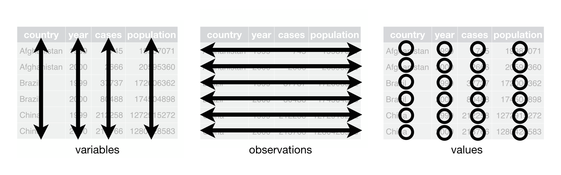
The defining opinion of the tidyverse is its wholehearted adoption of tidy data. Tidy data has three features:

Each variable forms a column.
Each observation forms a row.
Each type of observational unit forms a dataframe. (This is from the paper, not the book)

Tidy data was formalized by Hadley Wickham (2014) in the Journal of Statistical Software It is equivalent to Codd’s 3rd normal form (Codd, 1990) for relational databases.

Tidy datasets are all alike, but every messy dataset is messy in its own way. ~ Hadley Wickham

The tidy approach to data science is powerful because it breaks data work into two distinct parts. First, get the data into a tidy format. Second, use tools optimized for tidy data. By standardizing the data structure for most community-created tools, the framework oriented diffuse development and reduced the friction of data work.

2.4 dplyr

library(dplyr) contains workhorse functions for manipulating and summarizing data once it is in a tidy format. library(tidyr) contains functions for getting data into a tidy format.

dplyr can be explicitly loaded with library(dplyr) or loaded with library(tidyverse):

library(tidyverse)

We’ll focus on the key dplyr syntax using the March 2020 Annual Social and Economic Supplement (ASEC) to the Current Population Survey (CPS). Run the following code to load the data.

asec <- read_csv(
  paste0(
    "https://raw.githubusercontent.com/awunderground/awunderground-data/",
    "main/cps/cps-asec.csv"
  )
)

Rows: 157959 Columns: 17
── Column specification ────────────────────────────────────────────────────────
Delimiter: ","
chr  (4): month, ftype, offpov, offpovuniv
dbl (13): year, serial, cpsid, asecflag, asecwth, pernum, cpsidp, asecwt, ft...

ℹ Use `spec()` to retrieve the full column specification for this data.
ℹ Specify the column types or set `show_col_types = FALSE` to quiet this message.

We can use glimpse(asec) to quickly view the data. We can also use View(asec) to open up asec in RStudio.

glimpse(x = asec)

Rows: 157,959
Columns: 17
$ year       <dbl> 2020, 2020, 2020, 2020, 2020, 2020, 2020, 2020, 2020, 2020,…
$ serial     <dbl> 1, 1, 2, 2, 3, 4, 4, 5, 5, 5, 5, 7, 8, 9, 10, 10, 10, 12, 1…
$ month      <chr> "March", "March", "March", "March", "March", "March", "Marc…
$ cpsid      <dbl> 2.01903e+13, 2.01903e+13, 2.01812e+13, 2.01812e+13, 2.01902…
$ asecflag   <dbl> 1, 1, 1, 1, 1, 1, 1, 1, 1, 1, 1, 1, 1, 1, 1, 1, 1, 1, 1, 1,…
$ asecwth    <dbl> 1552.90, 1552.90, 990.49, 990.49, 1505.27, 1430.70, 1430.70…
$ pernum     <dbl> 1, 2, 1, 2, 1, 1, 2, 1, 2, 3, 4, 1, 1, 1, 1, 2, 3, 1, 2, 3,…
$ cpsidp     <dbl> 2.01903e+13, 2.01903e+13, 2.01812e+13, 2.01812e+13, 2.01902…
$ asecwt     <dbl> 1552.90, 1552.90, 990.49, 990.49, 1505.27, 1430.70, 1196.57…
$ ftype      <chr> "Primary family", "Primary family", "Primary family", "Prim…
$ ftotval    <dbl> 127449, 127449, 64680, 64680, 40002, 8424, 8424, 59114, 591…
$ inctot     <dbl> 52500, 74949, 44000, 20680, 40002, 0, 8424, 610, 58001, 503…
$ incwage    <dbl> 52500, 56000, 34000, 0, 40000, 0, 8424, 0, 58000, 0, 0, 0, …
$ offpov     <chr> "Above Poverty Line", "Above Poverty Line", "Above Poverty …
$ offpovuniv <chr> "In Poverty Universe", "In Poverty Universe", "In Poverty U…
$ offtotval  <dbl> 127449, 127449, 64680, 64680, 40002, 8424, 8424, 59114, 591…
$ offcutoff  <dbl> 17120, 17120, 17120, 17120, 13300, 15453, 15453, 26370, 263…

We’re going to learn seven functions and one new piece of syntax from library(dplyr) that will be our main tools for manipulating tidy frames. These functions and a few extensions outlined in the Data Transformation Cheat Sheet are the core of data analysis in the Tidyverse.

2.4.1 `select()`

select() drops columns from a dataframe and/or reorders the columns in a dataframe. The arguments after the name of the dataframe should be the names of columns you wish to keep, without quotes. All other columns not listed are dropped.

select(.data = asec, year, month, serial)

# A tibble: 157,959 × 3
    year month serial
   <dbl> <chr>  <dbl>
 1  2020 March      1
 2  2020 March      1
 3  2020 March      2
 4  2020 March      2
 5  2020 March      3
 6  2020 March      4
 7  2020 March      4
 8  2020 March      5
 9  2020 March      5
10  2020 March      5
# ℹ 157,949 more rows

This works great until the goal is to select 99 of 100 variables. Fortunately, - can be used to remove variables. You can also select all but multiple variables by listing them with the - symbol separated by commas.

select(.data = asec, -asecflag)

# A tibble: 157,959 × 16
    year serial month   cpsid asecwth pernum  cpsidp asecwt ftype ftotval inctot
   <dbl>  <dbl> <chr>   <dbl>   <dbl>  <dbl>   <dbl>  <dbl> <chr>   <dbl>  <dbl>
 1  2020      1 March 2.02e13   1553.      1 2.02e13  1553. Prim…  127449  52500
 2  2020      1 March 2.02e13   1553.      2 2.02e13  1553. Prim…  127449  74949
 3  2020      2 March 2.02e13    990.      1 2.02e13   990. Prim…   64680  44000
 4  2020      2 March 2.02e13    990.      2 2.02e13   990. Prim…   64680  20680
 5  2020      3 March 2.02e13   1505.      1 2.02e13  1505. Nonf…   40002  40002
 6  2020      4 March 2.02e13   1431.      1 2.02e13  1431. Prim…    8424      0
 7  2020      4 March 2.02e13   1431.      2 2.02e13  1197. Prim…    8424   8424
 8  2020      5 March 2.02e13   1133.      1 2.02e13  1133. Prim…   59114    610
 9  2020      5 March 2.02e13   1133.      2 2.02e13  1133. Prim…   59114  58001
10  2020      5 March 2.02e13   1133.      3 2.02e13  1322. Prim…   59114    503
# ℹ 157,949 more rows
# ℹ 5 more variables: incwage <dbl>, offpov <chr>, offpovuniv <chr>,
#   offtotval <dbl>, offcutoff <dbl>

Tidy data generally results in longer, wider data sets than other programming languages so iteratively selecting by column names is less important than in Stata or SAS. Still, dplyr contains powerful helper functions that can select variables based on patterns in column names:

contains(): Contains a given string
starts_with(): Starts with a prefix
ends_with(): Ends with a suffix
matches(): Matches a regular expression
num_range(): Matches a numerical range

These are a subset of the tidyselect selection language and helpers which enable users to apply library(dplyr) functions to select variables.

Exercise 1

Select pernum and inctot from asec.
pull() is related to select() but can only select one variable. What is the other difference with pull()?

2.4.2 `rename()`

rename() renames columns in a data frame. The pattern is new_name = old_name.

rename(.data = asec, serial_number = serial)

# A tibble: 157,959 × 17
    year serial_number month   cpsid asecflag asecwth pernum  cpsidp asecwt
   <dbl>         <dbl> <chr>   <dbl>    <dbl>   <dbl>  <dbl>   <dbl>  <dbl>
 1  2020             1 March 2.02e13        1   1553.      1 2.02e13  1553.
 2  2020             1 March 2.02e13        1   1553.      2 2.02e13  1553.
 3  2020             2 March 2.02e13        1    990.      1 2.02e13   990.
 4  2020             2 March 2.02e13        1    990.      2 2.02e13   990.
 5  2020             3 March 2.02e13        1   1505.      1 2.02e13  1505.
 6  2020             4 March 2.02e13        1   1431.      1 2.02e13  1431.
 7  2020             4 March 2.02e13        1   1431.      2 2.02e13  1197.
 8  2020             5 March 2.02e13        1   1133.      1 2.02e13  1133.
 9  2020             5 March 2.02e13        1   1133.      2 2.02e13  1133.
10  2020             5 March 2.02e13        1   1133.      3 2.02e13  1322.
# ℹ 157,949 more rows
# ℹ 8 more variables: ftype <chr>, ftotval <dbl>, inctot <dbl>, incwage <dbl>,
#   offpov <chr>, offpovuniv <chr>, offtotval <dbl>, offcutoff <dbl>

You can also rename a selection of variables using rename_with(). The .cols argument is used to select the columns to rename and takes a tidyselect statement like those we introduced above. Here, we’re using the where() selection helper which selects all columns where a given condition is TRUE. The default value for the .cols argument is everything() which selects all columns in the dataset.

rename_with(.data = asec, .fn = toupper, .cols = where(is.numeric))

# A tibble: 157,959 × 17
    YEAR SERIAL month   CPSID ASECFLAG ASECWTH PERNUM  CPSIDP ASECWT ftype      
   <dbl>  <dbl> <chr>   <dbl>    <dbl>   <dbl>  <dbl>   <dbl>  <dbl> <chr>      
 1  2020      1 March 2.02e13        1   1553.      1 2.02e13  1553. Primary fa…
 2  2020      1 March 2.02e13        1   1553.      2 2.02e13  1553. Primary fa…
 3  2020      2 March 2.02e13        1    990.      1 2.02e13   990. Primary fa…
 4  2020      2 March 2.02e13        1    990.      2 2.02e13   990. Primary fa…
 5  2020      3 March 2.02e13        1   1505.      1 2.02e13  1505. Nonfamily …
 6  2020      4 March 2.02e13        1   1431.      1 2.02e13  1431. Primary fa…
 7  2020      4 March 2.02e13        1   1431.      2 2.02e13  1197. Primary fa…
 8  2020      5 March 2.02e13        1   1133.      1 2.02e13  1133. Primary fa…
 9  2020      5 March 2.02e13        1   1133.      2 2.02e13  1133. Primary fa…
10  2020      5 March 2.02e13        1   1133.      3 2.02e13  1322. Primary fa…
# ℹ 157,949 more rows
# ℹ 7 more variables: FTOTVAL <dbl>, INCTOT <dbl>, INCWAGE <dbl>, offpov <chr>,
#   offpovuniv <chr>, OFFTOTVAL <dbl>, OFFCUTOFF <dbl>

Most dplyr functions can rename columns simply by prefacing the operation with new_name =. For example, this can be done with select():

select(.data = asec, year, month, serial_number = serial)

# A tibble: 157,959 × 3
    year month serial_number
   <dbl> <chr>         <dbl>
 1  2020 March             1
 2  2020 March             1
 3  2020 March             2
 4  2020 March             2
 5  2020 March             3
 6  2020 March             4
 7  2020 March             4
 8  2020 March             5
 9  2020 March             5
10  2020 March             5
# ℹ 157,949 more rows

2.4.3 `filter()`

filter() reduces the number of observations in a dataframe. Every column in a dataframe has a name. Rows do not necessarily have names in a dataframe, so rows need to be filtered based on logical conditions.

==, <, >, <=, >=, !=, %in%, and is.na() are all operators that can be used for logical conditions. ! can be used to negate a condition and & and | can be used to combine conditions. | means or.

# return rows with pernum of 1 and incwage > $100,000
filter(.data = asec, pernum == 1 & incwage > 100000)

# A tibble: 5,551 × 17
    year serial month   cpsid asecflag asecwth pernum  cpsidp asecwt ftype      
   <dbl>  <dbl> <chr>   <dbl>    <dbl>   <dbl>  <dbl>   <dbl>  <dbl> <chr>      
 1  2020     28 March 2.02e13        1    678.      1 2.02e13   678. Primary fa…
 2  2020    134 March 0              1    923.      1 0         923. Primary fa…
 3  2020    136 March 2.02e13        1    906.      1 2.02e13   906. Primary fa…
 4  2020    137 March 2.02e13        1   1493.      1 2.02e13  1493. Nonfamily …
 5  2020    359 March 2.02e13        1    863.      1 2.02e13   863. Primary fa…
 6  2020    372 March 2.02e13        1   1338.      1 2.02e13  1338. Primary fa…
 7  2020    404 March 0              1    677.      1 0         677. Primary fa…
 8  2020    420 March 2.02e13        1    747.      1 2.02e13   747. Primary fa…
 9  2020    450 March 2.02e13        1   1309.      1 2.02e13  1309. Primary fa…
10  2020    491 March 0              1   1130.      1 0        1130. Primary fa…
# ℹ 5,541 more rows
# ℹ 7 more variables: ftotval <dbl>, inctot <dbl>, incwage <dbl>, offpov <chr>,
#   offpovuniv <chr>, offtotval <dbl>, offcutoff <dbl>

IPUMS CPS contains full documentation with information about pernum and incwage.

Exercise 2

Filter asec to rows with month equal to "March".
Filter asec to rows with inctot less than 999999999.
Filter asec to rows with pernum equal to 3 and inctot less than 999999999.

2.4.4 `arrange()`

arrange() sorts the rows of a data frame in alpha-numeric order based on the values of a variable or variables. The dataframe is sorted by the first variable first and each subsequent variable is used to break ties. desc() is used to reverse the sort order for a given variable.

# sort pernum is descending order because high pernums are interesting
arrange(.data = asec, desc(pernum))

# A tibble: 157,959 × 17
    year serial month   cpsid asecflag asecwth pernum  cpsidp asecwt ftype      
   <dbl>  <dbl> <chr>   <dbl>    <dbl>   <dbl>  <dbl>   <dbl>  <dbl> <chr>      
 1  2020  91430 March 0              1    505.     16 0         604. Secondary …
 2  2020  91430 March 0              1    505.     15 0         465. Secondary …
 3  2020  91430 March 0              1    505.     14 0         416. Secondary …
 4  2020  15037 March 2.02e13        1   2272.     13 2.02e13  2633. Primary fa…
 5  2020  78495 March 0              1   1279.     13 0        1424. Related su…
 6  2020  91430 March 0              1    505.     13 0         465. Secondary …
 7  2020  15037 March 2.02e13        1   2272.     12 2.02e13  1689. Primary fa…
 8  2020  18102 March 0              1   2468.     12 0        2871. Primary fa…
 9  2020  22282 March 0              1   2801.     12 0        3879. Related su…
10  2020  30274 March 2.02e13        1    653.     12 2.02e13   858. Primary fa…
# ℹ 157,949 more rows
# ℹ 7 more variables: ftotval <dbl>, inctot <dbl>, incwage <dbl>, offpov <chr>,
#   offpovuniv <chr>, offtotval <dbl>, offcutoff <dbl>

Exercise 3

Sort asec in descending order by pernum and ascending order by inctot.

2.4.5 `mutate()`

mutate() creates new variables or edits existing variables. We can use arithmetic arguments, such as +, -, *, /, and ^. We can also custom functions and functions from packages. For example, we can use library(stringr) for string manipulation and library(lubridate) for date manipulation.

Variables are created by adding a new column name, like inctot_adjusted, to the left of = in mutate().

# adjust inctot for underreporting
mutate(.data = asec, inctot_adjusted = inctot * 1.1)

# A tibble: 157,959 × 18
    year serial month   cpsid asecflag asecwth pernum  cpsidp asecwt ftype      
   <dbl>  <dbl> <chr>   <dbl>    <dbl>   <dbl>  <dbl>   <dbl>  <dbl> <chr>      
 1  2020      1 March 2.02e13        1   1553.      1 2.02e13  1553. Primary fa…
 2  2020      1 March 2.02e13        1   1553.      2 2.02e13  1553. Primary fa…
 3  2020      2 March 2.02e13        1    990.      1 2.02e13   990. Primary fa…
 4  2020      2 March 2.02e13        1    990.      2 2.02e13   990. Primary fa…
 5  2020      3 March 2.02e13        1   1505.      1 2.02e13  1505. Nonfamily …
 6  2020      4 March 2.02e13        1   1431.      1 2.02e13  1431. Primary fa…
 7  2020      4 March 2.02e13        1   1431.      2 2.02e13  1197. Primary fa…
 8  2020      5 March 2.02e13        1   1133.      1 2.02e13  1133. Primary fa…
 9  2020      5 March 2.02e13        1   1133.      2 2.02e13  1133. Primary fa…
10  2020      5 March 2.02e13        1   1133.      3 2.02e13  1322. Primary fa…
# ℹ 157,949 more rows
# ℹ 8 more variables: ftotval <dbl>, inctot <dbl>, incwage <dbl>, offpov <chr>,
#   offpovuniv <chr>, offtotval <dbl>, offcutoff <dbl>, inctot_adjusted <dbl>

Variables are edited by including an existing column name, like inctot, to the left of = in mutate().

# adjust income because of underreporting
mutate(.data = asec, inctot = inctot * 1.1)

# A tibble: 157,959 × 17
    year serial month   cpsid asecflag asecwth pernum  cpsidp asecwt ftype      
   <dbl>  <dbl> <chr>   <dbl>    <dbl>   <dbl>  <dbl>   <dbl>  <dbl> <chr>      
 1  2020      1 March 2.02e13        1   1553.      1 2.02e13  1553. Primary fa…
 2  2020      1 March 2.02e13        1   1553.      2 2.02e13  1553. Primary fa…
 3  2020      2 March 2.02e13        1    990.      1 2.02e13   990. Primary fa…
 4  2020      2 March 2.02e13        1    990.      2 2.02e13   990. Primary fa…
 5  2020      3 March 2.02e13        1   1505.      1 2.02e13  1505. Nonfamily …
 6  2020      4 March 2.02e13        1   1431.      1 2.02e13  1431. Primary fa…
 7  2020      4 March 2.02e13        1   1431.      2 2.02e13  1197. Primary fa…
 8  2020      5 March 2.02e13        1   1133.      1 2.02e13  1133. Primary fa…
 9  2020      5 March 2.02e13        1   1133.      2 2.02e13  1133. Primary fa…
10  2020      5 March 2.02e13        1   1133.      3 2.02e13  1322. Primary fa…
# ℹ 157,949 more rows
# ℹ 7 more variables: ftotval <dbl>, inctot <dbl>, incwage <dbl>, offpov <chr>,
#   offpovuniv <chr>, offtotval <dbl>, offcutoff <dbl>

Conditional logic inside of mutate() with functions like if_else() and case_when() is key to mastering data munging in R.

Exercise 4

Create a new variable called in_poverty. If offtotval is less than offcutoff then use "Below Poverty Line". Otherwise, use "Above Poverty Line". Hint: if_else() is useful and works like the IF command in Microsoft Excel.

2.4.6 `|>`

Data munging is tiring when each operation needs to be assigned to a name with <-. The pipe, |>, allows lines of code to be chained together so the assignment operator only needs to be used once.

|> passes the output from function as the first argument in a subsequent function. For example, this line can be rewritten:

Legacy R code may use %>%, the pipe from the magrittr package. It was (and remains) wildly popular, particularly in the tidyverse framework. Due to this popularity, base R incorporated a similar concept in the base pipe. In many cases, these pipes work the same way, but there are some differences. Because |> is new and continues to be developed, developers have increased |>’s abilities over time. To see a list of key differences between %>% and |>, see this blog.

# old way
mutate(.data = asec, inctot_adjusted = inctot * 1.1)

# new way
asec |>
  mutate(inctot_adjusted = inctot * 1.1)

See the power:

new_asec <- asec |>
  filter(pernum == 1) |>
  select(year, month, pernum, inctot) |>
  mutate(inctot_adjusted = inctot * 1.1) |>
  select(-inctot)

new_asec

# A tibble: 60,460 × 4
    year month pernum inctot_adjusted
   <dbl> <chr>  <dbl>           <dbl>
 1  2020 March      1          57750 
 2  2020 March      1          48400 
 3  2020 March      1          44002.
 4  2020 March      1              0 
 5  2020 March      1            671 
 6  2020 March      1          19279.
 7  2020 March      1          12349.
 8  2020 March      1          21589.
 9  2020 March      1          47306.
10  2020 March      1          10949.
# ℹ 60,450 more rows

2.4.7 `summarize()`

summarize() collapses many rows in a dataframe into fewer rows with summary statistics of the many rows. n(), mean(), and sum() are common summary statistics. Renaming is useful with summarize()!

# summarize without renaming the statistics
asec |>
  summarize(mean(ftotval), mean(inctot))

# A tibble: 1 × 2
  `mean(ftotval)` `mean(inctot)`
            <dbl>          <dbl>
1         105254.     209921275.

# summarize and rename the statistics
asec |>
  summarize(mean_ftotval = mean(ftotval), mean_inctot = mean(inctot))

# A tibble: 1 × 2
  mean_ftotval mean_inctot
         <dbl>       <dbl>
1      105254.  209921275.

summarize() returns a data frame. This means all dplyr functions can be used on the output of summarize(). This is powerful! Manipulating summary statistics in Stata and SAS can be a chore. Here, it’s just another dataframe that can be manipulated with a tool set optimized for dataframes: dplyr.

2.4.8 `group_by()`

group_by() groups a dataframe based on specified variables. summarize() with grouped dataframes creates subgroup summary statistics. mutate() with group_by() calculates grouped summaries for each row.

asec |>
  group_by(pernum) |>
  summarize(
    n = n(),
    mean_ftotval = mean(ftotval), 
    mean_inctot = mean(inctot)
  )

# A tibble: 16 × 4
   pernum     n mean_ftotval mean_inctot
    <dbl> <int>        <dbl>       <dbl>
 1      1 60460       94094.      57508.
 2      2 45151      108700.   77497357.
 3      3 25650      117966.  473030618.
 4      4 15797      121815.  634999933.
 5      5  6752      108609.  691504650.
 6      6  2582       89448.  682810446.
 7      7   922       78889.  682218196.
 8      8   353       72284.  682725646.
 9      9   158       54599.  632917559.
10     10    73       58145.  657543632.
11     11    37       61847.  702708584 
12     12    18       50249.  777780725.
13     13     3       25152   666666666 
14     14     1       18000       18000 
15     15     1       25000       25000 
16     16     1       15000       15000

Dataframes can be grouped by multiple variables.

Grouped tibbles include metadata about groups. For example, Groups: pernum, offpov [40]. One grouping is dropped each time summarize() is used. It is easy to forget if a dataframe is grouped, so it is safe to include ungroup() at the end of a section of functions.

asec |>
  group_by(pernum, offpov) |>
  summarize(
    n = n(),
    mean_ftotval = mean(ftotval), 
    mean_inctot = mean(inctot)
  ) |>
  arrange(offpov) |>
  ungroup()

`summarise()` has grouped output by 'pernum'. You can override using the
`.groups` argument.

# A tibble: 40 × 5
   pernum offpov                 n mean_ftotval mean_inctot
    <dbl> <chr>              <int>        <dbl>       <dbl>
 1      1 Above Poverty Line 53872      104451.      63642.
 2      2 Above Poverty Line 40978      118691.   59082162.
 3      3 Above Poverty Line 23052      129891.  463440562.
 4      4 Above Poverty Line 14076      135039.  631720097.
 5      5 Above Poverty Line  5805      123937.  688206447.
 6      6 Above Poverty Line  2118      105867.  683199297.
 7      7 Above Poverty Line   724       96817.  697520661.
 8      8 Above Poverty Line   269       90328.  672870019.
 9      9 Above Poverty Line   114       70438.  622815186.
10     10 Above Poverty Line    57       71483.  666678408.
# ℹ 30 more rows

Exercise 5

filter() to only include observations with "In Poverty Universe" in offpovuniv.
group_by() offpov.
Use summarize() and n() to count the number of observations in poverty.

Exercise 6

filter() to only include observations with "In Poverty Universe".
group_by() cpsid.
Use mutate(family_size = n()) to calculate the family size for each observation in asec.
ungroup()
Create a new variable called in_poverty. If offtotval is less than offcutoff then use "Below Poverty Line". Otherwise, use "Above Poverty Line".
group_by() family_size, offpov, and in_poverty
Use summarize() and n() to see if you get the same result for offpov and in_poverty. You should only get two rows per family size if your poverty calculation is correct.

offcutoff comes from Census Bureau poverty tables with 48 unique thresholds based on family composition. Do not confuse the tables with HHS poverty tables.
These data come from IPUMS CPS. IPUMS has cleaned and pre-processed the data to include variables like offcutoff.

Are the estimates from the previous two exercises correct?

Let’s look at a Census Report to see how many people were in poverty in 2019. We estimated about 16,500 people. The Census Bureau says 34.0 million people.

No! We did not account for sampling weights, so our estimates are incorrect. Assignment 3 will demonstrate how to incorporate sampling weights into an analysis.

2.4.9 BONUS: `count()`

count() is a shortcut to df |> group_by(var) |> summarize(n()). count() counts the number of observations with a level of a variable or levels of several variables. It is too useful to skip:

count(asec, pernum)

# A tibble: 16 × 2
   pernum     n
    <dbl> <int>
 1      1 60460
 2      2 45151
 3      3 25650
 4      4 15797
 5      5  6752
 6      6  2582
 7      7   922
 8      8   353
 9      9   158
10     10    73
11     11    37
12     12    18
13     13     3
14     14     1
15     15     1
16     16     1

count(x = asec, pernum, offpov)

# A tibble: 40 × 3
   pernum offpov                 n
    <dbl> <chr>              <int>
 1      1 Above Poverty Line 53872
 2      1 Below Poverty Line  6588
 3      2 Above Poverty Line 40978
 4      2 Below Poverty Line  4156
 5      2 NIU                   17
 6      3 Above Poverty Line 23052
 7      3 Below Poverty Line  2527
 8      3 NIU                   71
 9      4 Above Poverty Line 14076
10      4 Below Poverty Line  1648
# ℹ 30 more rows

2.5 Mutating Joins

Mutating joins join one dataframe to columns from another dataframe by matching values common in both dataframes. The syntax is derived from Structured Query Language (SQL).

Each function requires an x (or left) dataframe, a y (or right) data frame, and by variables that exist in both dataframes. Note that below we’re creating dataframes using the tribble() function, which creates a tibble using a row-wise layout.

library(tidylog) is a useful function for monitoring the behavior of joins. It prints out summaries of the number of rows in each dataframe that successfully join.

math_scores <- tribble(
  ~name, ~math_score,
  "Alec", 95,
  "Bart", 97,
  "Carrie", 100
)

reading_scores <- tribble(
  ~name, ~reading_score,
  "Alec", 88,
  "Bart", 67,
  "Carrie", 100,
  "Zeta", 100
)

2.5.1 `left_join()`

left_join() matches observations from the y dataframe to the x dataframe. It only keeps observations from the y data frame that have a match in the x dataframe.

left_join(x = math_scores, y = reading_scores, by = "name")

# A tibble: 3 × 3
  name   math_score reading_score
  <chr>       <dbl>         <dbl>
1 Alec           95            88
2 Bart           97            67
3 Carrie        100           100

Observations that exist in the x (left) dataframe but not in the y (right) dataframe result in NAs.

left_join(x = reading_scores, y = math_scores, by = "name")

# A tibble: 4 × 3
  name   reading_score math_score
  <chr>          <dbl>      <dbl>
1 Alec              88         95
2 Bart              67         97
3 Carrie           100        100
4 Zeta             100         NA

2.5.2 `inner_join()`

inner_join() matches observations from the y dataframe to the x dataframe. It only keeps observations from either data frame that have a match.

inner_join(x = reading_scores, y = math_scores, by = "name")

# A tibble: 3 × 3
  name   reading_score math_score
  <chr>          <dbl>      <dbl>
1 Alec              88         95
2 Bart              67         97
3 Carrie           100        100

2.5.3 `full_join()`

full_join() matches observations from the y dataframe to the x dataframe. It keeps observations from both dataframes.

full_join(x = reading_scores, y = math_scores, by = "name")

# A tibble: 4 × 3
  name   reading_score math_score
  <chr>          <dbl>      <dbl>
1 Alec              88         95
2 Bart              67         97
3 Carrie           100        100
4 Zeta             100         NA

2.6 Filtering Joins

Filtering joins drop observations based on the presence of their key (identifier) in another data frame. They use the same syntax as mutating joins with an x (or left) dataframe, a y (or right) data frame, and by variables that exist in both dataframes.

2.6.1 `anti_join()`

anti_join() returns all rows from x where there are not matching values in y. anti_join() complements inner_join(). Together, they should exhaust the x dataframe.

anti_join(x = reading_scores, y = math_scores, by = "name")

# A tibble: 1 × 2
  name  reading_score
  <chr>         <dbl>
1 Zeta            100

Note

The Combine Tables column in the Data Transformation Cheat Sheet is an invaluable resource for navigating joins. The “column matching for joins” section of that cheat sheet outlines how to join tables by matching on multiple columns or match on columns with different names in each table.

R for Data Science (2e) also has an excellent chapter covering joins.

2.7 readr

readr is a core tidyverse package for reading and parsing rectangular data from text files (.csv, .tsv, etc.). read_csv() reads .csv files and has a bevy of advantages versus read.csv(). We recommend never using read.csv().

Many .csvs can be read without issue with simple syntax read_csv(file = "relative/path/to/data").

readr and read_csv() have powerful tools for resolving parsing issues. More can be learned in the data import section in R for Data Science (2e).

2.8 readxl

readxl is a tidyverse package for reading data from Microsoft Excel files. It is not a core tidyverse package so it needs to be explicitly loaded in each R session.

We introduce the package more thoroughly in Section 3.2.2. The tidyverse website has a good tutorial on readxl.

2.9 Conclusion

This chapter introduced tidy data in which columns reflect a variable, observations reflect a row, and cells reflect an individual observation. It also introduced key functions from dplyr, a tidyverse package built to support data cleaning operations:

select() for removing columns
filter() for removing rows
rename() for renaming columns
arrange() for reordering columns
mutate() for creating new columns
|> (the pipe operator) for chaining together multiple functions (part of base, but extremely useful!)
summarize() for collapsing many rows of a data frame into fewer rows
group_by() to group a data frame by certain specified variables
count() a shortcut for group_by() |> summarize(n())

The chapter also introduced mutating joins (left_join(), inner_join(), and full_join()) which create new columns and filtering joins (anti_join()) which drop observations depending on the presence of their key in another data frame.

The chapter concluded by introducing the readr and readxl packages which are useful for reading data into R.

2.9.1 Next Skills

across() can be used with library(dplyr) functions such as summarise() and mutate() to apply the same transformations to multiple columns. For example, it can be used to calculate the mean of many columns with summarize(). across() uses the same tidyselect select language and helpers discussed earlier to select the columns to transform.
pivot_wider() and pivot_longer() can be used to switch between wide and long formats of the data. This is important for tidying data and data visualization.

2.1 Review

2.1.1 Assignment operator

2.2 Functions

2.2.1 == vs. =

2.3 Tidy data

2.3.1 tidyverse

2.3.2 Opinionated software

2.3.3 Tidy data

2.4 dplyr

2.4.1 select()

2.4.2 rename()

2.4.3 filter()

2.4.4 arrange()

2.4.5 mutate()

2.4.6 |>

2.4.7 summarize()

2.4.8 group_by()

2.4.9 BONUS: count()

2.5 Mutating Joins

2.5.1 left_join()

2.5.2 inner_join()

2.5.3 full_join()

2.6 Filtering Joins

2.6.1 anti_join()

2.7 readr

2.8 readxl

2.9 Conclusion

2.9.1 Next Skills

2.2.1 `==` vs. `=`

2.4.1 `select()`

2.4.2 `rename()`

2.4.3 `filter()`

2.4.4 `arrange()`

2.4.5 `mutate()`

2.4.6 `|>`

2.4.7 `summarize()`

2.4.8 `group_by()`

2.4.9 BONUS: `count()`

2.5.1 `left_join()`

2.5.2 `inner_join()`

2.5.3 `full_join()`

2.6.1 `anti_join()`