# A tibble: 58,077 × 2
   gutenberg_id text
          <int> <chr>
 1         1404 "THE FEDERALIST PAPERS"
 2         1404 "THE FEDERALIST PAPERS"
 3         1404 "THE FEDERALIST PAPERS"
 4         1404 ""
 5         1404 ""
 6         1404 ""
 7         1404 "By Alexander Hamilton, John Jay, and James Madison"
 8         1404 "By Alexander Hamilton, John Jay, and James Madison"
 9         1404 "By Alexander Hamilton, John Jay, and James Madison"
10         1404 ""
# ℹ 58,067 more rows25 Text Analysis
Abstract
In this chapter, we introduce fundamental ideas for text analysis.
Image by Raysonho
25.1 Motivation
Before providing motivation, let’s define two key terms.
TipText Corpus
A set of text. A corpus generally has theme such as “The Federalist Papers” or Jane Austin novels.
TipText analysis
The process of deriving information from text using algorithms and statistical analysis.
Text analysis has broad applications that extend well beyond policy analysis. We will briefly focus on four applications that are related to policy analysis.
25.1.1 1. Document Summarization
The process of condensing the amount of information in a document into a useful subset of information. Techniques range from counting words to using complex machine learning algorithms.
Example: Frederick Mosteller and David Wallace used Bayesian statistics and the frequency of certain words to identify the authorship of the twelve unclaimed Federalist papers. (blog) Before estimating any models, they spent months cutting out each word of the Federalist Papers and the counting the frequency of words.
25.1.2 2. Text Classification (supervised)
The process of labeling documents with a predetermined set of labels.
Example: Researchers in the Justice Policy Center at the Urban Institute classified millions of tweets with the word “cop” or “police” as “positive”, “negative”, “neutral”, or “not applicable” for sentiment and “crime or incident information”, “department or event information”, “traffic or weather updates”, “person identification”, or “other” for topic. The researchers created content and metadata features, manually labeled a few thousand tweets for training data, and used gradient boosting for supervised machine learning for the task. (blog)
Example: Frederick Mosteller and David Wallace used Bayesian statistics and the frequency of certain words to identify the authorship of the twelve unclaimed Federalist papers. (blog)
25.1.3 3. Document Grouping (unsupervised)
The algorithmic grouping or clustering of documents using features extracted from the documents. This includes unsupervised classification of documents into meaningful groups. Techniques like topic modeling result in lists of important words that can be used to summarize and label the documents while techniques like K-means clustering result in arbitrary cluster labels.
Example: Pew Research used unsupervised and semi-supervised methods to create topic models of open-ended text responses about where Americans find meaning in their lives. (blog)
25.1.4 4. Text Extraction
Text often contains important unstructured information that would be useful to have in a structured format like a table. Text extraction is the process of searching and identifying key entities or concepts from unstructured text and then placing them in a structured format.
Example: Researchers from Cornell counted sources of misinformation from 38 million articles. NYTimes. Methodology.
25.1.5 Other
Speech recognition, machine translation, question answering, and text autocompletion are other forms of text analysis and language processing that are common but not implemented with R packages.
25.2 Tools
25.2.1 Frequency
TipTerm Frequency
A count or relative frequency of the most common words in a document or documents.
TipTerm Frequency-Inverse Document Frequency (TF-IDF)
Some words are naturally more common than other words. TF-IDF quantifies the importance of words/terms in one document relative to other documents in a corpus.
\[TF-IDF = TF(t, d) \cdot IDF(t)\]
where \(TF(t, d)\) is the relative frequency of term \(t\) in document \(d\) and \(IDF(t)\) is the inverse frequency of the number of document where the term appears.
\[TF-IDF = \frac{f_{t, d}}{\sum_{t' \in d} f_{t', d}} \cdot \left(\log\left(\frac{1 + n}{1 + df(d, f)}\right) + 1\right)\]
TipWord cloud
A method of visualizing word frequency where the frequency of a given word is encoded as the size of the word.
Word clouds are overused and are tough to interpret. This 2016 election word cloud by Gallup is an exceptional word cloud.
25.2.2 Collocation
TipN-gram
A consecutive sequence of n words. Unigrams are words, bigrams are pairs of words, and trigrams are groups of three words.
TipN-gram frequency
A count or relative frequency of n-grams in a document or documents.
TipTF-IDF of N-grams
TF-IDF with n-grams instead of words.
TipBigram graph
A directed or undirected graph with individual words as nodes and bigrams as edges. Example
25.3 Topic Modeling
TipTopic modeling
Unsupervised and semi-supervised methods for grouping documents. Example
Popular methods include:
- Latent Dirichlet Allocation (LDA)
- Non-Negative Matrix Factorization
- CorEx (Correlation Explanation)
25.4 Natural Language Processing
TipNatural language processing
The algorithmic analysis of text in a way that is rooted in linguistics. Stanford CoreNLP is an important tool for natural language processing.
TipSentiment analysis
The process of labeling words or sentences as positive, neutral, or negative.
TipNamed entity recognition
The process of identifying names, places, organizations, and more in text.
TipParts of speech tagging
The process of identifying the part of speech of each word (noun, verb, etc.).
TipLemmatization
The process of shortening words to a base grammar.
25.4.1 Key Challenge
R and Python have powerful tools for text analysis.
Key challenge: text contains a lot of useful information but its structure does not match how we have done data analysis up to this point.
25.5 Vocabulary & Tidy Data
TipToken
A meaningful unit of text. Tokens include works, phrases, and sentences.
TipTokenization
Process of splitting a larger unit of text into tokens. For example, “data science is useful” can be “data”, “science”, “is”, “useful”.
# A tibble: 1,297 × 2
   gutenberg_id word
          <int> <chr>
 1         1404 by
 2         1404 alexander
 3         1404 hamilton
 4         1404 john
 5         1404 jay
 6         1404 and
 7         1404 james
 8         1404 madison
 9         1404 by
10         1404 alexander
# ℹ 1,287 more rows
TipStemming
A method of removing the end, and keeping only the root, of a word. Stemming is unaware of the context or use of the word. Example
# A tibble: 471 × 3
   gutenberg_id word         stem
          <int> <chr>        <chr>
 1         1404 alexander    alexand
 2         1404 jay          jai
 3         1404 james        jame
 4         1404 alexander    alexand
 5         1404 jay          jai
 6         1404 james        jame
 7         1404 general      gener
 8         1404 introduction introduct
 9         1404 general      gener
10         1404 introduction introduct
# ℹ 461 more rows
TipLemmatizing
A method of returning the base of a word. Lemmatization considers the context of a word. Example Lemmatizing requires natural language processing, so this requires Stanford CoreNLP or the Python package spaCy, which can be accessed in R via library(spacyr).
TipStop words
Extremely common words that are often not useful for text analysis. library(tidytext) contains stop words from the onix, SMART, and snowball lexicons.
# A tibble: 1,149 × 2
   word        lexicon
   <chr>       <chr>
 1 a           SMART
 2 a's         SMART
 3 able        SMART
 4 about       SMART
 5 above       SMART
 6 according   SMART
 7 accordingly SMART
 8 across      SMART
 9 actually    SMART
10 after       SMART
# ℹ 1,139 more rows
TipTidy text
A table with one token per row.” ~ Text Mining with R
Text can also be stored as a string, a corpus, and a document-term matrix.
25.6 Example 1
# load necessary packages
library(tidyverse)
library(tidytext)
library(gutenbergr)
library(SnowballC)

# download the Federalist Papers from Project Gutenberg
fed_papers <- gutenberg_download(
  gutenberg_id = 1404,
  mirror = "http://mirror.csclub.uwaterloo.ca/gutenberg"
)

# this data cleaning comes from Emil Hvitfeldt
# https://www.hvitfeldt.me/blog/predicting-authorship-in-the-
# federalist-papers-with-tidytext/
hamilton <- c(1, 6:9, 11:13, 15:17, 21:36, 59:61, 65:85)
madison <- c(10, 14, 18:20, 37:48)
jay <- c(2:5, 64)
unknown <- c(49:58, 62:63)

fed_papers <- pull(fed_papers, text) |>
  str_c(collapse = " ") |>
  str_split(pattern = "\\.|\\?|\\!") |>
  unlist() %>%
  tibble(text = .) |>
  mutate(sentence = row_number())

tidy_fed_papers <- fed_papers |>
  mutate(
    paper_number = cumsum(
      str_detect(
        text,
        regex("FEDERALIST No", ignore_case = TRUE)))
  ) |>
  unnest_tokens(word, text) |>
  mutate(
    author = case_when(
      paper_number %in% hamilton ~ "hamilton",
      paper_number %in% madison ~ "madison",
      paper_number %in% jay ~ "jay",
      paper_number %in% unknown ~ "unknown"
    )
  )
25.6.1 Approach 1
Here we’ll calculate term frequency without stop words and with stemming.
# filter to main authors
tidy_fed_papers1 <- tidy_fed_papers |>
  filter(author %in% c("hamilton", "madison"))

# remove stop words and stem the words
tidy_fed_papers1 <- tidy_fed_papers1 |>
  anti_join(stop_words, by = "word") |>
  mutate(word = wordStem(word))

# count Hamilton's most-frequent words
tidy_fed_papers1 |>
  filter(author == "hamilton") |>
  count(word, sort = TRUE)
# A tibble: 2,728 × 2
word n
<chr> <int>
1 govern 648
2 nation 510
3 peopl 363
4 power 360
5 union 315
6 time 234
7 author 198
8 danger 192
9 confederaci 186
10 countri 183
# ℹ 2,718 more rows# A tibble: 1,592 × 2
word n
<chr> <int>
1 govern 174
2 nation 153
3 union 108
4 power 96
5 war 81
6 confederaci 69
7 peopl 69
8 form 63
9 object 63
10 time 63
# ℹ 1,582 more rows25.6.2 Approach 2
Here we’ll perform TF-IDF.
Warning: A value for tf_idf is negative:
 Input should have exactly one row per document-term combination.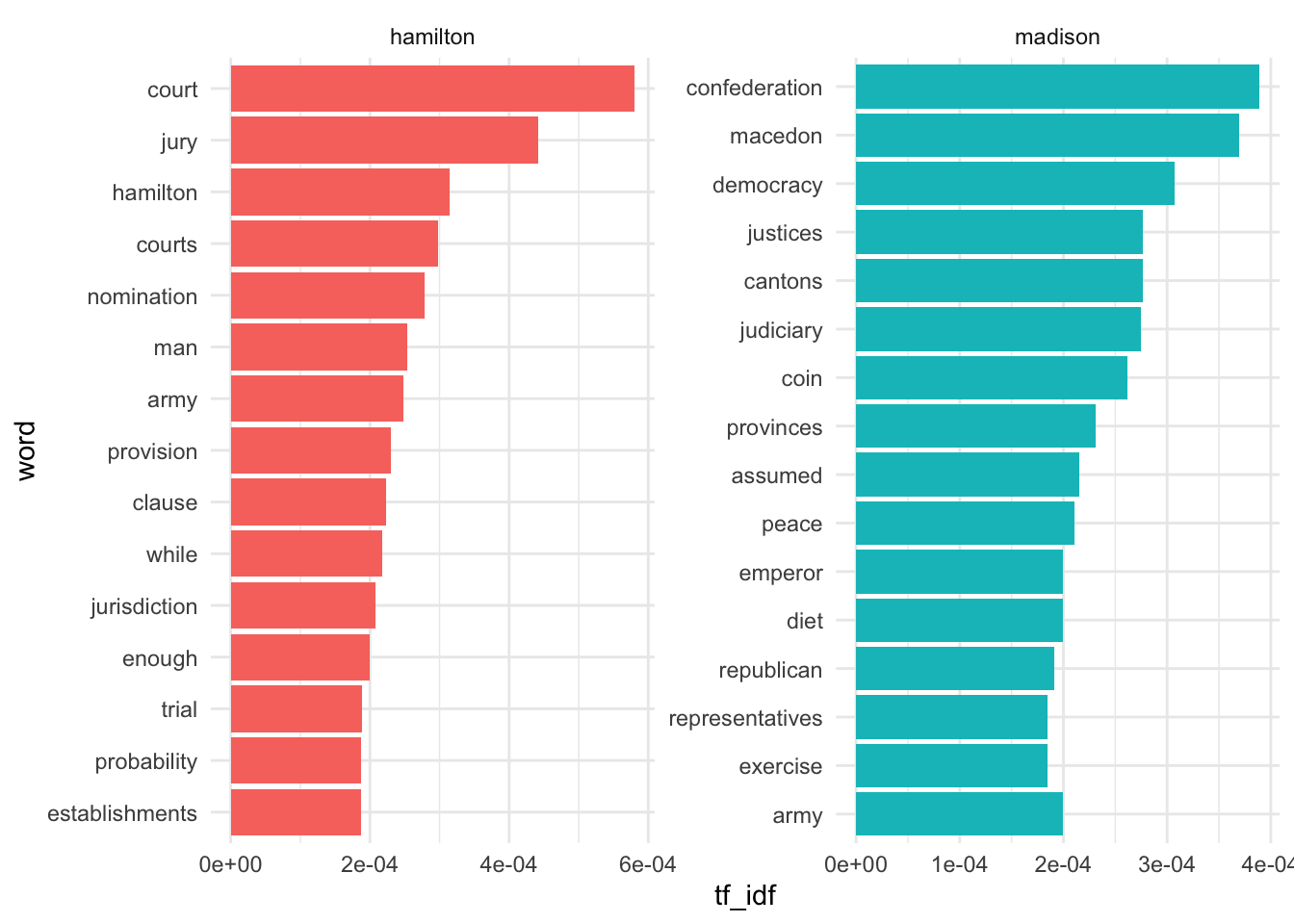
25.6.3 Approach 3
25.7 Example 2
Let’s consider ten of Shakespeare’s plays.
ids <- c(
  2265, # Hamlet
  1795, # Macbeth
  1522, # Julius Caesar
  2235, # The Tempest
  1780, # 1 Henry IV
  1532, # King Lear
  1513, # Romeo and Juliet
  1110, # King John
  1519, # Much Ado About Nothing
  1539  # The Winter's Tale
)

# download corpus
shakespeare <- gutenberg_download(
  gutenberg_id = ids,
  mirror = "https://www.gutenberg.org/",
  meta_fields = "title"
)

# create tokens and drop character cues
shakespeare_clean <- shakespeare |>
  unnest_tokens(word, text, to_lower = FALSE) |>
  filter(word != str_to_upper(word))

# calculate TF-IDF
shakespeare_tf_idf <- shakespeare_clean |>
  count(title, word, sort = TRUE) |>
  bind_tf_idf(term = word, document = title, n = n)

# plot
shakespeare_tf_idf |>
  group_by(title) |>
  top_n(8, tf_idf) |>
  mutate(word = reorder(word, tf_idf)) |>
  ggplot(aes(tf_idf, word, fill = title)) +
  geom_col() +
  facet_wrap(~title, scales = "free", ncol = 2) +
  theme_minimal() +
  guides(fill = "none")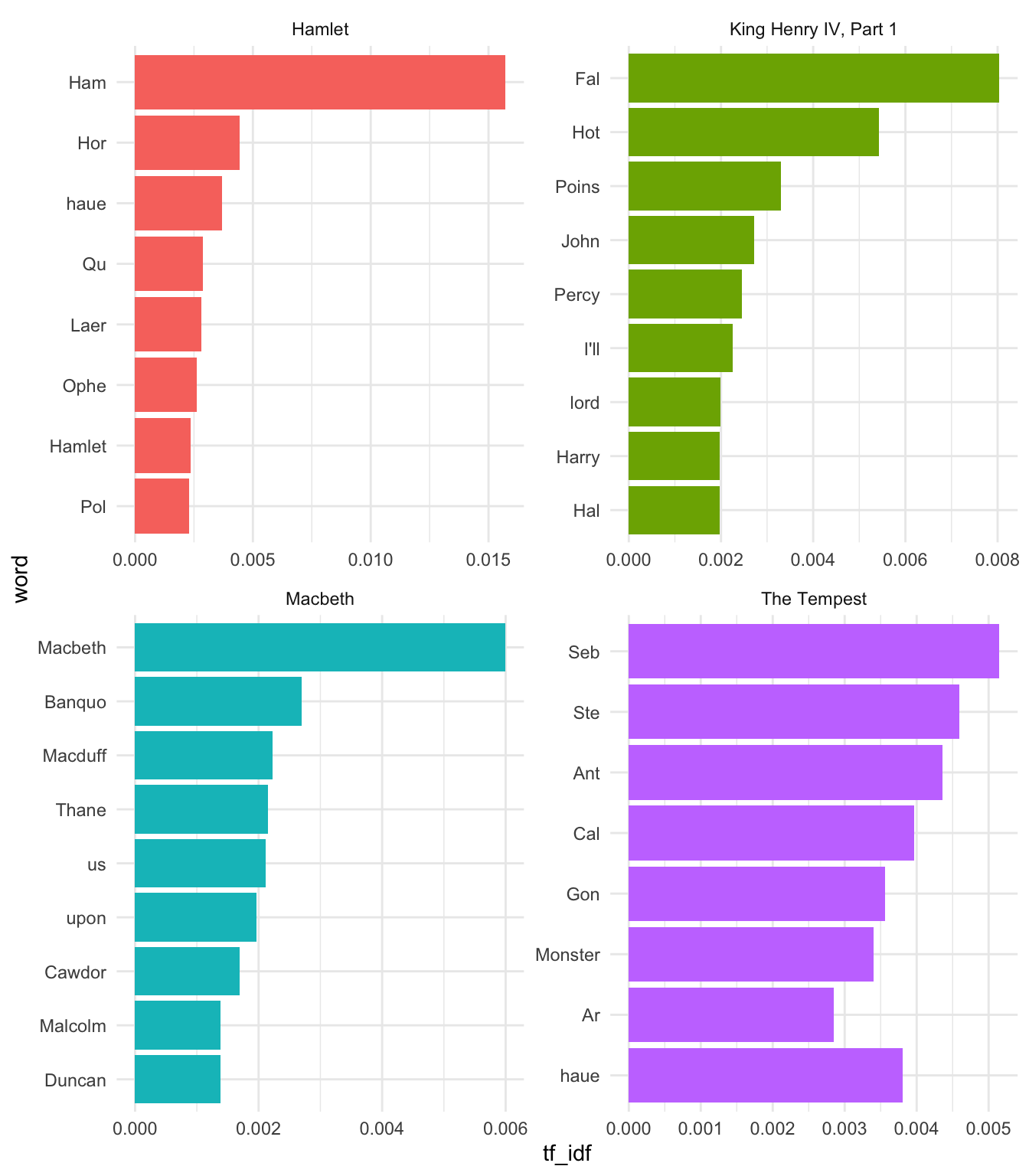
25.8 Resources
- Corporate Reporting in the Era of Artificial Intelligence
- Text Mining with R by Julia Silge and David Robinson
- Supervised Machine Learning for Text Analysis in R by Emil Hvitfledt and Julia Silge
- Corpus