| true_value | predicted_value |
|---|---|
| 0 | 0 |
| 0 | 0 |
| 0 | 0 |
| 1 | 0 |
| 1 | 1 |
| 1 | 1 |
| 0 | 1 |
| 0 | 1 |
| 1 | 1 |
| 1 | 1 |
19 Classification
19.1 Types of Classification
Binary classification: Predicting one of two classes. For example, rat burrow or no rat burrow, lead paint or no lead paint, or insured or uninsured. Classes are often recoded to 1 and 0 as in logistic regression.
Multiclass classification: Predicting one of three or more classes. For example, single filer, joint filer, or head of household; or on-time, delinquent, or defaulted. Classes can be recoded to integers for models like multinomial logistic regression, but many of the best models can handle factors.
19.2 Metrics
Classification problems require a different set of error metrics and diagnostics than regression problems. Assume a binary classifier for the following definitions. Let an event be the outcome 1 in a binary classification problem and a non-event be the outcome 0.
True positive: Correctly predicting an event. Predicting \(\hat{y_i} = 1\) when \(y_i = 1\)
True negative: Correctly predicting a non-event. Predicting \(\hat{y_i} = 0\) when \(y_i = 0\)
False positive: Incorrectly predicting an event for a non-event. Predicting \(\hat{y_i} = 1\) when \(y_i = 0\)
False negative: Incorrectly predicting a non-event for an event. Predicting \(\hat{y_i} = 0\) when \(y = 1\)
Confusion matrix: A simple matrix that compares predicted outcomes with actual outcomes.
As these notes will show, there are many ways to combine true positives, false positives, true negatives, and false negatives into a given metric. It is important to understand a use-case in which a predictive algorithm will be used. That should inform the specific metric selected.
| True Value | |||
| \(y=1\) | \(y=0\) | ||
| Predicted Value | \(\hat{y}=1\) | True Positive (TP) | False Positive (FP) |
| \(\hat{y}=0\) | False Negative (FN) | True Negative (TN) |
Accuracy: The sum of the values on the main diagonal of the confusion matrix divided by the total number of predictions (\(\frac{TP + TN}{total}\)).
19.2.1 Example 1
Consider the following set of true values and predicted values from a binary classification problem:
The confusion matrix for this data:
| True Value | |||
| \(y=1\) | \(y=0\) | ||
| Predicted Value | \(\hat{y}=1\) | 4 | 2 |
| \(\hat{y}=0\) | 1 | 3 |
19.2.2 Example 2
A test for breast cancer is 99.1% accurate across 1,000 tests. Is it a good test?
| True Value | |||
| \(y=1\) | \(y=0\) | ||
| Predicted Value | \(\hat{y}=1\) | 1 | 4 |
| \(\hat{y}=0\) | 5 | 990 |
This test only accurately predicted one cancer case. In fact, a person was more likely not to have cancer given a positive test than to have cancer. This example demonstrates the base rate fallacy and the accuracy paradox. Both are the results of high class imbalance. Clearly we need more sophisticated way of evaluating classifiers than just accuracy.
19.3 More metrics
19.3.1 Most Important Metrics
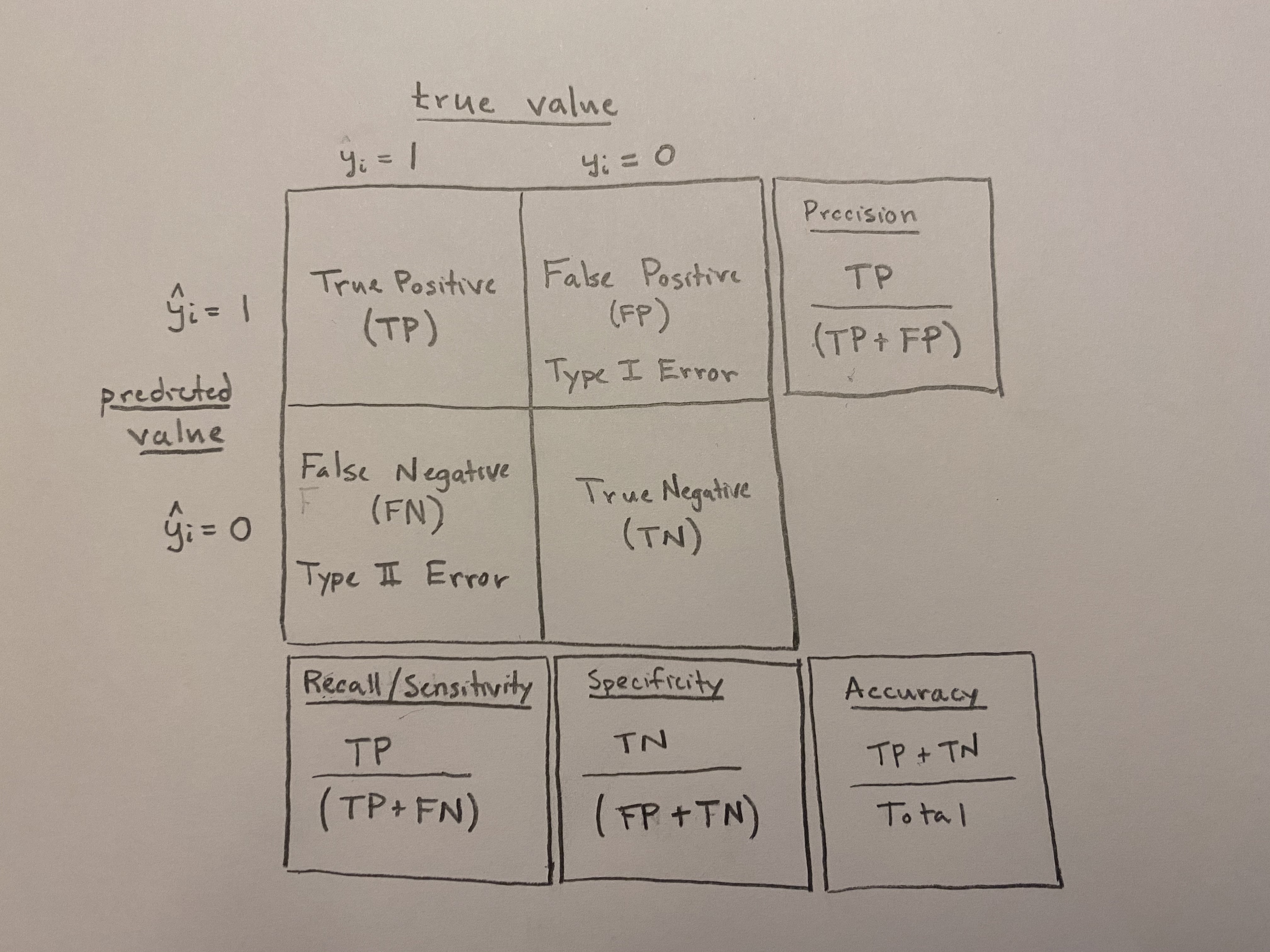
Accuracy: How often the classifier is correct. \(\frac{TP +TN}{total}\). All else equal, we want to maximize accuracy.
Precision: How often the classifier is correct when it predicts events. \(\frac{TP}{TP+FP}\). All else equal, we want to maximize precision.
Recall/Sensitivity/True Positive Rate: How often the classifier is correct when there is an event. \(\frac{TP}{TP+FN}\). All else equal, we want to maximize recall/sensitivity.
19.3.2 Other Metrics
Specificity: How often the classifier is correct when there is a non-event. \(\frac{TN}{TN+FP}\). All else equal, we want to maximize specificity.
False Positive Rate: 1 - Specificity
Note that False Positive Rate is sometimes referred to as FPR.
19.3.3 Example 2 continued
| True Value | |||
| \(y=1\) | \(y=0\) | ||
| Predicted Value | \(\hat{y}=1\) | 1 | 4 |
| \(\hat{y}=0\) | 5 | 990 |
Precision: \(\frac{TP}{TP + FP} = \frac{1}{1 + 4} = \frac{1}{5}\)
Recall/Sensitivity: \(\frac{TP}{TP + FN} = \frac{1}{1 + 5} = \frac{1}{6}\)
The breast cancer test has poor precision and recall.
Specificity: \(\frac{TN}{FP + TN} = \frac{990}{4 + 990} = \frac{990}{994}\)
False Positive Rate (FPR): \(1 - Specificity = \frac{4}{994}\)
The breast cancer cancer test also has poor False Positive Rate.
19.3.4 Using Thresholds to Predict Classes:
Most algorithms for classification generate predicted classes and probabilities of predicted classes. A predicted probability of 0.99 for an event is very different than a predicted probability of 0.51.
To generate class predictions, usually a threshold is used. For example, if \(\hat{P}(event) > 0.5\) then predict event. It is common to adjust the threshold to values other than 0.5. As 0.5 decreases, marginal cases shift from \(\hat{y} = 0\) to \(\hat{y} = 1\) because the threshold for an event decreases.
As the threshold decreases (we are predicting more events and fewer non-events):
- the true positive rate increases and the false positive rate increases
- precision decreases and sensitivity/recall increases
- sensitivity increases and specificity decreases
In general, the goal is to create a model that has a high true positive rate and a low false positive rate, high precision and high recall, and high sensitivity and high specificity. Changing the threshold is a movement along these tradeoffs. Estimating “better” models is often a way to improve these tradeoffs. Of course, there is some amount of irreducible error.
Receiver Operating Characteristics (ROC) curve: A curve that shows the trade-off between the false positive rate and true positive rate as different threshold probabilities are used for classification.
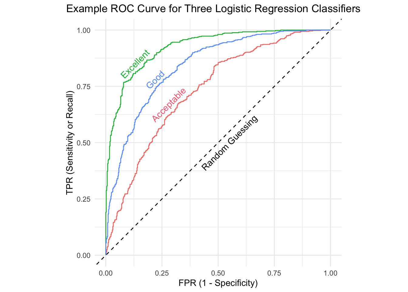
Area Under the Curve (AUC): A one-number summary of an ROC curve where 0.5 is random guessing and the rules of thumb are 0.7 is acceptable, 0.8 is good, and 0.9 is excellent.
AUC is also sometimes referred to as AUROC (Area under the Receiver Operating Curve).
# A tibble: 3 × 4
  Quality    .metric .estimator .estimate
  <chr>      <chr>   <chr>          <dbl>
1 Acceptable roc_auc binary         0.733
2 Good       roc_auc binary         0.841
3 Excellent roc_auc binary 0.92519.3.5 Relative costs
True positives, true negatives, false positives, and false negatives can carry different costs, and it is important to consider the relative costs when creating models and interventions.
A false positive for a cancer test could result in more diagnostic tests. A false negative for a cancer test could lead to untreated cancer and severe health consequences. The relative differences in these outcomes should be considered.
A false positive for a rat burrow is a wasted trip for an exterminator. A false negative for an rat burrow is an untreated rat burrow. The difference in these outcomes is small, especially compared to the alternative of the exterminator guessing which alleys to visit.
19.3.6 Multiclass metrics
Consider a multiclass classification problem with three unique levels (“a”, “b”, “c”)
| true_value | predicted_value |
|---|---|
| a | a |
| a | a |
| a | a |
| a | a |
| b | b |
| b | a |
| b | b |
| b | c |
| c | c |
| c | b |
| c | a |
| c | c |
Create a confusion matrix:
| True Value | ||||
|---|---|---|---|---|
| \(y=a\) | \(y=b\) | \(y=c\) | ||
| Predicted Value | \(\hat{y}=a\) | 4 | 1 | 1 |
| \(\hat{y}=b\) | 0 | 2 | 2 | |
| \(\hat{y}=c\) | 0 | 1 | 2 |
Accuracy still measures how often the classifier is correct. In multiclass classification problem, the correct predictions are on the diagonal.
Accuracy: \(\frac{4 + 2 + 2}{12} = \frac{8}{12} = \frac{2}{3}\)
There are multiclass extensions of precision, recall/sensitivity, and specificity. They are beyond the scope of this class.
19.4 R Code
19.4.1 Example 1
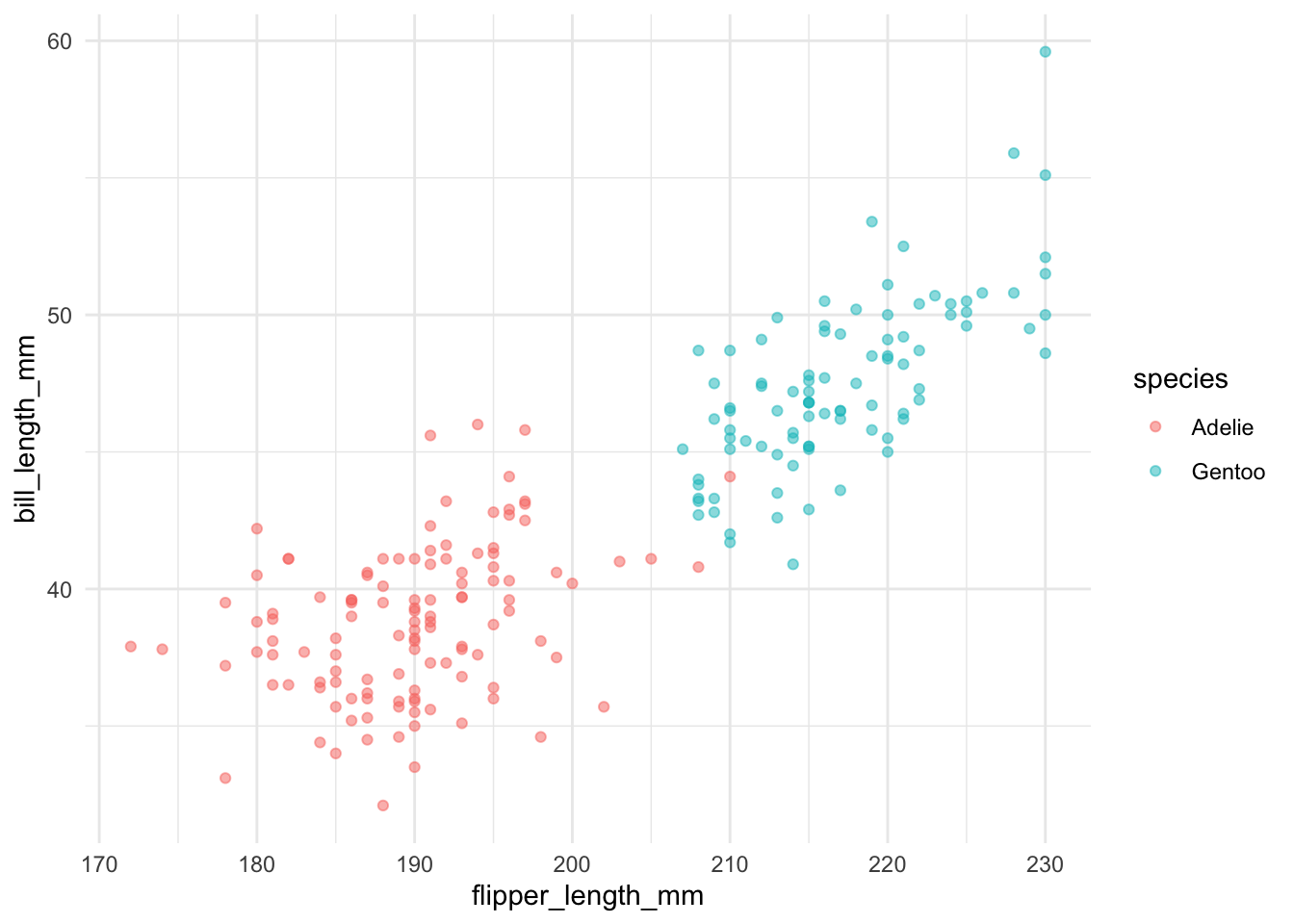
Example 1 uses data about penguins from the Palmer Archipelago in Antarctica. The data include measurements about three different species of penguins. This example only considers two classes and does not use resampling methods because only one model is estimated.
          species            island    bill_length_mm     bill_depth_mm
                0                 0                 2                 2
flipper_length_mm       body_mass_g               sex              year
2 2 11 0 Step 1. Split the data into training and testing data
Step 2. EDA
Step 3. Estimate a Model
# create a recipe
cart_rec <-
  recipe(formula = species ~ ., data = penguins_small_train)

# create a cart model object
cart_mod <-
  decision_tree() %>%
  set_engine(engine = "rpart") %>%
  set_mode(mode = "classification")

cart_wf <- workflow() %>%
  add_recipe(cart_rec) %>%
  add_model(cart_mod)

# fit the model
cart_fit <- cart_wf %>%
  fit(data = penguins_small_train)

# create a tree
rpart.plot::rpart.plot(x = cart_fit$fit$fit$fit)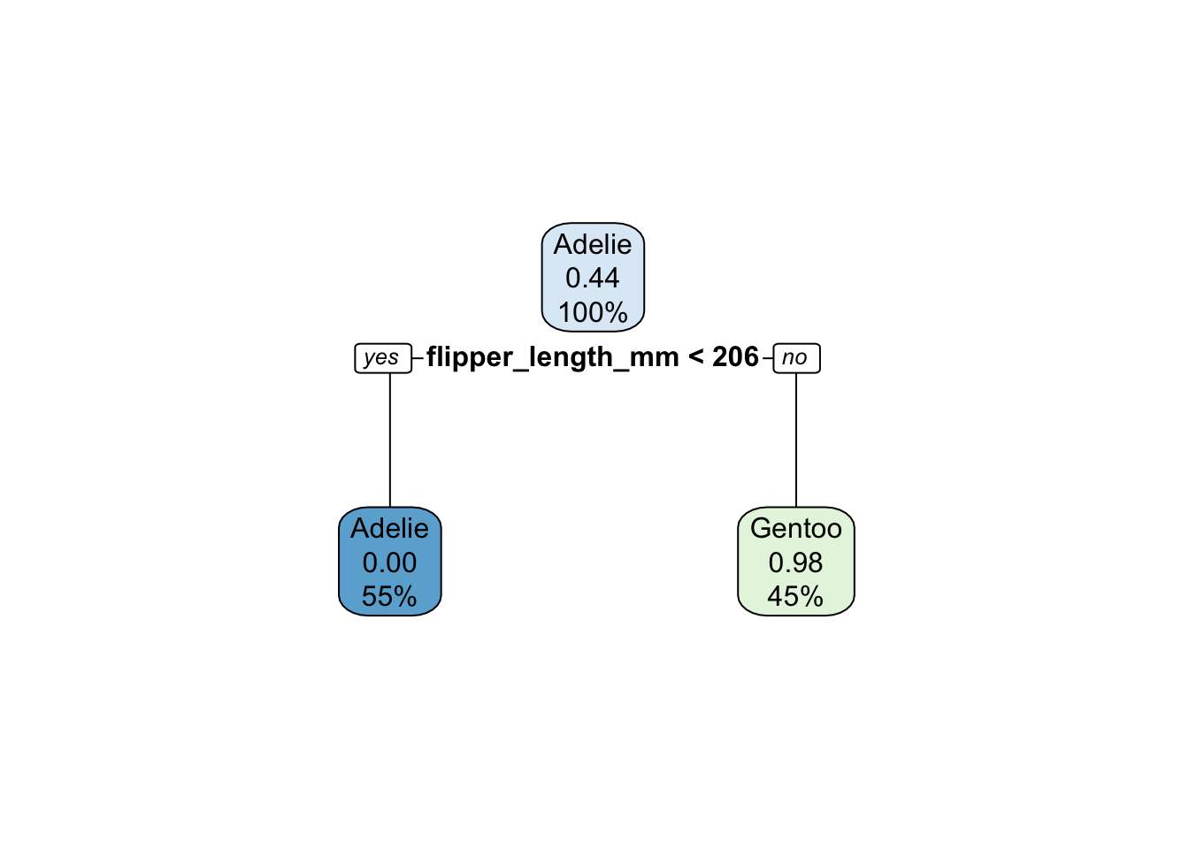
Step 4. Evaluate a Model
# predict the predicted class and the predicted probability of each class
predictions <- bind_cols(
  penguins_small_test,
  predict(object = cart_fit, new_data = penguins_small_test),
  predict(object = cart_fit, new_data = penguins_small_test, type = "prob")
)

select(predictions, species, starts_with(".pred"))
# A tibble: 53 × 4
species .pred_class .pred_Adelie .pred_Gentoo
<fct> <fct> <dbl> <dbl>
1 Adelie Adelie 1 0
2 Adelie Adelie 1 0
3 Adelie Adelie 1 0
4 Adelie Adelie 1 0
5 Adelie Adelie 1 0
6 Adelie Adelie 1 0
7 Adelie Adelie 1 0
8 Adelie Adelie 1 0
9 Adelie Adelie 1 0
10 Adelie Adelie 1 0
# ℹ 43 more rowsCreate a confusion matrix:
Step 5. Make a New Prediction
# A tibble: 1 × 1
  .pred_class
  <fct>
1 Adelie # A tibble: 1 × 2
.pred_Adelie .pred_Gentoo
<dbl> <dbl>
1 1 0Note that the decision tree has one split, on flipper length. Below the threshold, all penguins are Adelie. Consequently, the probability associated with .pred_Adelie is 100% or 1.0. You can see this with the code below:
