3 Advanced Data Cleaning

Abstract

This section covers advanced techniques for cleaning and manipulating data using the tidyverse.

3.1 Review

R for Data Science (2e) displays the first steps of the data science process as “Import”, “Tidy”, and “Transform”. Recall from the previous lecture techniques for importing data like read_csv() and for transforming data like mutate().

Exercise 1

Use mutate() and case_when() to add a new variable called speed_cat to cars where the values are "slow" when speed < 10, "moderate" when speed < 20, and "fast" otherwise.

In the last lecture, we introduced mutating joins and filtering joins.

Mutating Joins

Mutating joins add new variables to a data frame by matching observations from one data frame to observations in another data frame.

Filtering Joins

Filtering joins drop observations based on the presence of their key (identifier) in another data frame.

For example, we may have a list of students in detention and a list of all students. We can use a filtering join to create a list of student not in detention.

Let their be two data frames x and y and let both data frames have a key variable that uniquely identifies rows. In practice, in R, we often use the following functions:

left_join(x, y) appends variables from y on to x but only keeps observations from x.
inner_join(x, y) appends variables from y onto x but only keeps observations for which there is a match between the x and ydata frames.
full_join(x, y) appends variables from y on to x and keeps all observations from x and y.
anti_join(x, y) returns all observations from x without a match in y. anti_join() is traditionally only used for filtering joins, but it is useful for writing tests for mutating joins.

To learn more, read the joins chapter of R for Data Science (2e).

3.2 Import

3.2.1 `library(here)`

Developing Quarto documents in subdirectories is a pain. When interactively running code in the console, file paths are read as if the .qmd file is in the same folder as the .Rproj. When clicking render, paths are treated as if they are in the subdirectory where the .qmd file is.

library(here) resolves headaches around file referencing in project-oriented workflows.

Loading library(here) will print your working directory.

library(here)

here() starts at /Users/aaronwilliams/presentations/data-science-for-public-policy2

After this, here() will use reasonable heuristics to find project files using relative file paths. When placing Quarto documents in a directory below the top-level directory, use here() and treat each folder and file as a different string.

Before

read_csv("data/raw/important-data.csv")

After

read_csv(here("data", "raw", "important-data.csv"))

3.2.2 `library(readxl)`

We will focus on reading data from Excel workbooks. Excel is a bad tool with bad design that has led to many analytical errors. Unfortunately, it’s a dominant tool for storing data and often enters the data science workflow.

library(readxl) is the premier package for reading data from .xls and .xlsx files. read_excel(), which works like read_csv(), loads data from .xls and .xlsx files. Consider data from the Urban Institute’s Debt in America feature accessed through the Urban Institute Data Catalog.

library(readxl)

read_excel(here("data", "state_dia_delinquency_ 7 Jun 2022.xlsx"))

# A tibble: 51 × 28
   fips  state_name          state Share with Any Debt …¹ Share with Any Debt …²
   <chr> <chr>               <chr> <chr>                  <chr>                 
 1 01    Alabama             AL    .3372881               .5016544              
 2 02    Alaska              AK    .1672429               .221573               
 3 04    Arizona             AZ    .2666938               .3900013              
 4 05    Arkansas            AR    .3465793               .5426918              
 5 06    California          CA    .2087713               .2462195              
 6 08    Colorado            CO    .213803                .3554938              
 7 09    Connecticut         CT    .2194708               .3829038              
 8 10    Delaware            DE    .2866829               .469117               
 9 11    District of Columb… DC    .2232908               .3485817              
10 12    Florida             FL    .2893825               .3439322              
# ℹ 41 more rows
# ℹ abbreviated names: ¹`Share with Any Debt in Collections, All`,
#   ²`Share with Any Debt in Collections, Communities of Color`
# ℹ 23 more variables:
#   `Share with Any Debt in Collections, Majority White Communities` <chr>,
#   `Median Debt in Collections, All` <chr>,
#   `Median Debt in Collections, Communities of Color` <chr>, …

read_excel() has several useful arguments:

sheet selects the sheet to read.
range selects the cells to read and can use Excel-style ranges like “C34:D50”.
skip skips the selected number of rows.
n_max selects the maximum number of rows to read.

Excel encourages bad habits and untidy data, so these arguments are useful for extracting data from messy Excel workbooks.

readxl_example() contains a perfect example. The workbook contains two sheets, which we can see with excel_sheets().

readxl_example("clippy.xlsx") |>
  excel_sheets()

[1] "list-column"    "two-row-header"

As is common with many Excel workbooks, the second sheet contains a second row of column names with parenthetical comments about each column.¹

readxl_example("clippy.xlsx") |>  
  read_excel(sheet = "two-row-header")

# A tibble: 2 × 4
  name       species              death                 weight    
  <chr>      <chr>                <chr>                 <chr>     
1 (at birth) (office supply type) (date is approximate) (in grams)
2 Clippy     paperclip            39083                 0.9

This vignette suggests a simple solution to this problem.

# extract the column names
col_names <- readxl_example("clippy.xlsx") |>  
  read_excel(sheet = "two-row-header", n_max = 0) |>
  names()

# load the data and add the column names
readxl_example("clippy.xlsx") |>  
    read_excel(
      sheet = "two-row-header", 
      skip = 2,
      col_names = col_names
    )

# A tibble: 1 × 4
  name   species   death               weight
  <chr>  <chr>     <dttm>               <dbl>
1 Clippy paperclip 2007-01-01 00:00:00    0.9

Exercise 2

The IRS Statistics of Income Division is one of the US’s 13 principal statistical agencies. They publish rich information derived from tax returns. We will focus on Table 1, Adjusted Gross Income (AGI) percentiles by state.

Read in the 52 cells in the first column that contain “United States”, all 50 states, and the “District of Columbia”.
Identify the cells containing data for “Adjusted gross income floor on percentiles”. Read in the data with read_excel(). Either programmatically read in the column names (i.e. “Top 1 Percent”, …) or assign them with col_names().
Use bind_cols() to combine the data from step 1 and step 2.

library(tidyxl) contains tools for working with messy Excel workbooks, library(openxlsx) contains tools for creating Excel workbooks with R, and library(googlesheets4) contains tools for working with Google Sheets.

3.3 Tidy

The defining opinion of the tidyverse is its wholehearted adoption of tidy data. Tidy data has three features:

Each variable forms a column.
Each observation forms a row.
Each type of observational unit forms a dataframe.

Tidy datasets are all alike, but every messy dataset is messy in its own way. ~ Hadley Wickham

library(tidyr) is the main package for tidying untidy data. We’ll practice some skills using examples from three workbooks from the IRS SOI.

pivot_longer() is commonly used for tidying data and for making data longer for library(ggplot2). pivot_longer() reorients data so that key-value pairs expressed as column name-column value are column value-column value in adjacent columns. pivot_longer() has three essential arguments:

cols is a vector of columns to pivot (or not pivot).
names_to is a string for the name of the column where the old column names will go (i.e. “series” in the figure).
values_to is a string for the name of the column where the values will go (i.e. “rate” in the figure).

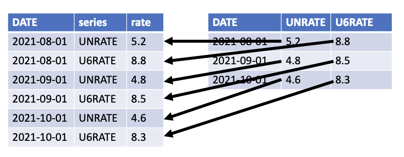
pivot_wider() is the inverse of pivot_longer().

Why aren’t the data tidy?

table1 <- tribble(
  ~state, ~agi2006, ~agi2016, ~agi2020,
  "Alabama", 95067, 114510, 138244,
  "Alaska", 17458, 23645, 26445,
  "Arizona", 146307, 181691, 245258
)

table1

# A tibble: 3 × 4
  state   agi2006 agi2016 agi2020
  <chr>     <dbl>   <dbl>   <dbl>
1 Alabama   95067  114510  138244
2 Alaska    17458   23645   26445
3 Arizona  146307  181691  245258

Year is a variable. This data is untidy because year is included in the column names.

table1 <- tribble(
  ~state, ~agi2006, ~agi2016, ~agi2020,
  "Alabama", 95067, 114510, 138244,
  "Alaska", 17458, 23645, 26445,
  "Arizona", 146307, 181691, 245258
)

table1

# A tibble: 3 × 4
  state   agi2006 agi2016 agi2020
  <chr>     <dbl>   <dbl>   <dbl>
1 Alabama   95067  114510  138244
2 Alaska    17458   23645   26445
3 Arizona  146307  181691  245258

pivot_longer(
  data = table1, 
  cols = -state, 
  names_to = "year", 
  values_to = "agi"
)

# A tibble: 9 × 3
  state   year       agi
  <chr>   <chr>    <dbl>
1 Alabama agi2006  95067
2 Alabama agi2016 114510
3 Alabama agi2020 138244
4 Alaska  agi2006  17458
5 Alaska  agi2016  23645
6 Alaska  agi2020  26445
7 Arizona agi2006 146307
8 Arizona agi2016 181691
9 Arizona agi2020 245258

The year column isn’t useful yet. We’ll fix that later.

library(tidyr) contains several functions to split values into multiple cells.

separate_wider_delim() separates a value based on a delimeter and creates wider data.
separate_wider_position() separates a value based on position and creates wider data.
separate_longer_delim() separates a value based on a delimeter and creates longer data.
separate_longer_position() separates a value based on position and creates longer data.

Tidying Example 2

Untidy
Cleaned

Why aren’t the data tidy?

table2 <- tribble(
  ~state, ~`agi2006|2016|2020`,
  "Alabama", "95067|114510|138244",
  "Alaska", "17458|23645|26445",
  "Arizona", "146307|181691|245258"
)

table2

# A tibble: 3 × 2
  state   `agi2006|2016|2020` 
  <chr>   <chr>               
1 Alabama 95067|114510|138244 
2 Alaska  17458|23645|26445   
3 Arizona 146307|181691|245258

The values for 2006, 2016, and 2020 are all squished into one cell.

table2 <- tribble(
  ~state, ~`agi2006|2016|2020`,
  "Alabama", "95067|114510|138244",
  "Alaska", "17458|23645|26445",
  "Arizona", "146307|181691|245258"
)

table2

# A tibble: 3 × 2
  state   `agi2006|2016|2020` 
  <chr>   <chr>               
1 Alabama 95067|114510|138244 
2 Alaska  17458|23645|26445   
3 Arizona 146307|181691|245258

separate_wider_delim(
  data = table2, 
  cols = `agi2006|2016|2020`, 
  delim = "|",
  names = c("2006", "2016", "2020")
) |>
  pivot_longer(
    cols = -state,
    names_to = "year", 
    values_to = "agi"
  )

# A tibble: 9 × 3
  state   year  agi   
  <chr>   <chr> <chr> 
1 Alabama 2006  95067 
2 Alabama 2016  114510
3 Alabama 2020  138244
4 Alaska  2006  17458 
5 Alaska  2016  23645 
6 Alaska  2020  26445 
7 Arizona 2006  146307
8 Arizona 2016  181691
9 Arizona 2020  245258

bind_rows() combines data frames by stacking the rows.

one <- tribble(
  ~id, ~var,
  "1", 3.14,
  "2", 3.15,
)

two <- tribble(
  ~id, ~var,
  "3", 3.16,
  "4", 3.17,
)

bind_rows(one, two)

# A tibble: 4 × 2
  id      var
  <chr> <dbl>
1 1      3.14
2 2      3.15
3 3      3.16
4 4      3.17

bind_cols() combines data frames by appending columns.

three <- tribble(
  ~id, ~var1,
  "1", 3.14,
  "2", 3.15,
)

four <- tribble(
  ~id, ~var2,
  "1", 3.16,
  "2", 3.17,
)

bind_cols(three, four)

New names:
• `id` -> `id...1`
• `id` -> `id...3`

# A tibble: 2 × 4
  id...1  var1 id...3  var2
  <chr>  <dbl> <chr>  <dbl>
1 1       3.14 1       3.16
2 2       3.15 2       3.17

When possible, we recommend using relational joins like left_join() to combine by columns because it is easy to miss-align rows with bind_cols().

left_join(
  x = three,
  y = four,
  by = "id"
)

# A tibble: 2 × 3
  id     var1  var2
  <chr> <dbl> <dbl>
1 1      3.14  3.16
2 2      3.15  3.17

Tidying Example 3

Untidy
Cleaned

Why aren’t the data tidy?

table3_2006 <- tribble(
  ~state, ~agi,
  "Alabama", "95067",
  "Alaska", "17458",
  "Arizona", "146307"
)

table3_2006

# A tibble: 3 × 2
  state   agi   
  <chr>   <chr> 
1 Alabama 95067 
2 Alaska  17458 
3 Arizona 146307

table3_2016 <- tribble(
  ~state, ~agi,
  "Alabama", "114510",
  "Alaska", "23645",
  "Arizona", "181691"
)

table3_2016

# A tibble: 3 × 2
  state   agi   
  <chr>   <chr> 
1 Alabama 114510
2 Alaska  23645 
3 Arizona 181691

table3_2020 <- tribble(
  ~state, ~`agi`,
  "Alabama", "138244",
  "Alaska", "26445",
  "Arizona", "245258"
)

table3_2020

# A tibble: 3 × 2
  state   agi   
  <chr>   <chr> 
1 Alabama 138244
2 Alaska  26445 
3 Arizona 245258

The variable year is contained in the data set names. The .id argument in bind_rows() allows us to create the year variable.

table3_2006 <- tribble(
  ~state, ~agi,
  "Alabama", 95067,
  "Alaska", 17458,
  "Arizona", 146307
)

table3_2006

# A tibble: 3 × 2
  state      agi
  <chr>    <dbl>
1 Alabama  95067
2 Alaska   17458
3 Arizona 146307

table3_2016 <- tribble(
  ~state, ~agi,
  "Alabama", 114510,
  "Alaska", 23645,
  "Arizona", 181691
)

table3_2016

# A tibble: 3 × 2
  state      agi
  <chr>    <dbl>
1 Alabama 114510
2 Alaska   23645
3 Arizona 181691

table3_2020 <- tribble(
  ~state, ~`agi`,
  "Alabama", 138244,
  "Alaska", 26445,
  "Arizona", 245258
)

table3_2020

# A tibble: 3 × 2
  state      agi
  <chr>    <dbl>
1 Alabama 138244
2 Alaska   26445
3 Arizona 245258

bind_rows(
  `2006` = table3_2006,
  `2016` = table3_2016,
  `2020` = table3_2020,
  .id = "year"
)

# A tibble: 9 × 3
  year  state      agi
  <chr> <chr>    <dbl>
1 2006  Alabama  95067
2 2006  Alaska   17458
3 2006  Arizona 146307
4 2016  Alabama 114510
5 2016  Alaska   23645
6 2016  Arizona 181691
7 2020  Alabama 138244
8 2020  Alaska   26445
9 2020  Arizona 245258

Relational joins are fundamental to working with tidy data. Tidy data can only contain one unit of observation (e.g. county or state not county and state). When data exist on multiple levels, they must be stored in separate tables that can later be combined.

Tidying Example 4

Untidy
Cleaned

Why aren’t the data tidy?

table4a <- tribble(
  ~state, ~agi,
  "Alabama", 95067,
  "Alaska", 17458,
  "Arizona", 146307
)

table4a

# A tibble: 3 × 2
  state      agi
  <chr>    <dbl>
1 Alabama  95067
2 Alaska   17458
3 Arizona 146307

table4b <- tribble(
  ~state, ~returns,
  "Alabama", 1929941,
  "Alaska", 322369,
  "Arizona", 2454951
)

table4b

# A tibble: 3 × 2
  state   returns
  <chr>     <dbl>
1 Alabama 1929941
2 Alaska   322369
3 Arizona 2454951

These data are tidy! But keeping the data in two separate data frames may not make sense. Let’s use full_join() to combine the data and anti_join() to see if there are mismatches.

table4a <- tribble(
  ~state, ~agi,
  "Alabama", 95067,
  "Alaska", 17458,
  "Arizona", 146307
)

table4a

# A tibble: 3 × 2
  state      agi
  <chr>    <dbl>
1 Alabama  95067
2 Alaska   17458
3 Arizona 146307

table4b <- tribble(
  ~state, ~returns,
  "Alabama", 1929941,
  "Alaska", 322369,
  "Arizona", 2454951
)

table4b

# A tibble: 3 × 2
  state   returns
  <chr>     <dbl>
1 Alabama 1929941
2 Alaska   322369
3 Arizona 2454951

full_join(table4a, table4b, by = "state")

# A tibble: 3 × 3
  state      agi returns
  <chr>    <dbl>   <dbl>
1 Alabama  95067 1929941
2 Alaska   17458  322369
3 Arizona 146307 2454951

anti_join(table4a, table4b, by = "state")

# A tibble: 0 × 2
# ℹ 2 variables: state <chr>, agi <dbl>

anti_join(table4b, table4a, by = "state")

# A tibble: 0 × 2
# ℹ 2 variables: state <chr>, returns <dbl>

Exercise 3

Use pivot_longer() to make the SOI percentile data from the earlier exercise longer. After the transformation, there should be one row per percentile per state.

To see more examples, read the tidy data section in R for Data Science (2e)

3.4 Transform

3.4.1 Strings

Check out the stringr cheat sheet.

library(stringr) contains powerful functions for working with strings in R. In data analysis, we may need to detect matches, subset strings, work with the lengths of strings, modify strings, and join and split strings.

Detecting Matches

str_detect() is useful for detecting matches in strings, which can be useful with filter(). Consider the executive orders data set and suppose we want to return executive orders that contain the word "Virginia".

eos <- read_csv(here("data", "executive-orders.csv")) |>
  filter(!is.na(text)) |>
  group_by(executive_order_number) |>
  summarize(text = list(text)) |>
  mutate(text = map_chr(text, ~paste(.x, collapse = " ")))

Rows: 196537 Columns: 4
── Column specification ────────────────────────────────────────────────────────
Delimiter: ","
chr  (2): text, president
dbl  (1): executive_order_number
date (1): signing_date

ℹ Use `spec()` to retrieve the full column specification for this data.
ℹ Specify the column types or set `show_col_types = FALSE` to quiet this message.

eos

# A tibble: 1,126 × 2
   executive_order_number text                                                  
                    <dbl> <chr>                                                 
 1                  12890 "Executive Order 12890 of December 30, 1993 Amendment…
 2                  12944 "Executive Order 12944 of December 28, 1994 Adjustmen…
 3                  12945 "Executive Order 12945 of January 20, 1995 Amendment …
 4                  12946 "Executive Order 12946 of January 20, 1995 President'…
 5                  12947 "Executive Order 12947 of January 23, 1995 Prohibitin…
 6                  12948 "Executive Order 12948 of January 30, 1995 Amendment …
 7                  12949 "Executive Order 12949 of February 9, 1995 Foreign In…
 8                  12950 "Executive Order 12950 of February 22, 1995 Establish…
 9                  12951 "Executive Order 12951 of February 22, 1995 Release o…
10                  12952 "Executive Order 12952 of February 24, 1995 Amendment…
# ℹ 1,116 more rows

eos |>
  filter(str_detect(string = text, pattern = "Virginia"))

# A tibble: 6 × 2
  executive_order_number text                                                   
                   <dbl> <chr>                                                  
1                  13150 Executive Order 13150 of April 21, 2000 Federal Workfo…
2                  13508 Executive Order 13508 of May 12, 2009 Chesapeake Bay P…
3                  13557 Executive Order 13557 of November 4, 2010 Providing an…
4                  13775 Executive Order 13775 of February 9, 2017 Providing an…
5                  13787 Executive Order 13787 of March 31, 2017 Providing an O…
6                  13934 Executive Order 13934 of July 3, 2020 Building and Reb…

Subsetting Strings

str_sub() can subset strings based on positions within the string. Consider an example where we want to extract state FIPS codes from county FIPS codes.

tibble(fips = c("01001", "02013", "04001")) |>
  mutate(state_fips = str_sub(fips, start = 1, end = 2))

# A tibble: 3 × 2
  fips  state_fips
  <chr> <chr>     
1 01001 01        
2 02013 02        
3 04001 04

Managing Lengths

str_pad() is useful for managing lengths. Consider the common situation when zeros are dropped from the beginning of FIPS codes.

tibble(fips = c(1, 2, 4)) |>
  mutate(fips = str_pad(fips, side = "left", pad = "0", width = 2))

# A tibble: 3 × 1
  fips 
  <chr>
1 01   
2 02   
3 04

Modifying Strings

str_replace(), str_replace_all(), str_remove(), and str_remove_all() can delete or modify parts of strings. Consider an example where we have course names and we want to delete everything except numeric digits.²

tibble(course = c("PPOL 670", "GOVT 8009", "PPOL 6819")) |>
  mutate(course = str_remove(course, pattern = "[:alpha:]*\\s"))

# A tibble: 3 × 1
  course
  <chr> 
1 670   
2 8009  
3 6819

str_c() and str_glue() are useful for joining strings. Consider an example where we want to “fill in the blank” with a variable in a data frame.

tibble(fruit = c("apple", "banana", "cantelope")) |>
  mutate(sentence = str_glue("my favorite fruit is {fruit}"))

# A tibble: 3 × 2
  fruit     sentence                      
  <chr>     <glue>                        
1 apple     my favorite fruit is apple    
2 banana    my favorite fruit is banana   
3 cantelope my favorite fruit is cantelope

tibble(fruit = c("apple", "banana", "cantelope")) |>
  mutate(
    another_sentence = 
      str_c("Who doesn't like a good ", fruit, ".")
    )

# A tibble: 3 × 2
  fruit     another_sentence                  
  <chr>     <chr>                             
1 apple     Who doesn't like a good apple.    
2 banana    Who doesn't like a good banana.   
3 cantelope Who doesn't like a good cantelope.

This workflow is useful for building up URLs when accessing APIs, scraping information from the Internet, and downloading many files.

Exercise 4

Use mutate() and library(stringr) to create a variable for year from the earlier SOI exercise. For instance, "agi2006" should be "2006".
Use as.numeric() to convert the string from step 1 into a numeric value.
Create a data visualization with year on the x-axis.

3.4.2 Factors {sec-factors}

Check out the forcats cheat sheet.

Much of our work focuses on four of the six types of atomic vectors: logical, integer, double, and character. R also contains augmented vectors like factors.

Factors are categorical data stored as integers with a levels attribute. Character vectors often work well for categorical data and many of R’s functions convert character vectors to factors. This happens with lm().

Factors have many applications:

Giving the levels of a categorical variable non-alpha numeric order in a ggplot2 data visualization.
Running calculations on data with empty groups.
Representing categorical outcome variables in classification models.

Factor Basics

x1 <- factor(c("a", "a", "b", "c"), levels = c("d", "c", "b", "a"))

x1

[1] a a b c
Levels: d c b a

attributes(x1)

$levels
[1] "d" "c" "b" "a"

$class
[1] "factor"

levels(x1)

[1] "d" "c" "b" "a"

x1 has order but it isn’t ordinal. Sometimes we’ll come across ordinal factor variables, like with the diamonds data set. Unintentional ordinal variables can cause unexpected errors. For example, including ordinal data as predictors in regression models will lead to different estimated coefficients than other variable types.

glimpse(diamonds)

Rows: 53,940
Columns: 10
$ carat   <dbl> 0.23, 0.21, 0.23, 0.29, 0.31, 0.24, 0.24, 0.26, 0.22, 0.23, 0.…
$ cut     <ord> Ideal, Premium, Good, Premium, Good, Very Good, Very Good, Ver…
$ color   <ord> E, E, E, I, J, J, I, H, E, H, J, J, F, J, E, E, I, J, J, J, I,…
$ clarity <ord> SI2, SI1, VS1, VS2, SI2, VVS2, VVS1, SI1, VS2, VS1, SI1, VS1, …
$ depth   <dbl> 61.5, 59.8, 56.9, 62.4, 63.3, 62.8, 62.3, 61.9, 65.1, 59.4, 64…
$ table   <dbl> 55, 61, 65, 58, 58, 57, 57, 55, 61, 61, 55, 56, 61, 54, 62, 58…
$ price   <int> 326, 326, 327, 334, 335, 336, 336, 337, 337, 338, 339, 340, 34…
$ x       <dbl> 3.95, 3.89, 4.05, 4.20, 4.34, 3.94, 3.95, 4.07, 3.87, 4.00, 4.…
$ y       <dbl> 3.98, 3.84, 4.07, 4.23, 4.35, 3.96, 3.98, 4.11, 3.78, 4.05, 4.…
$ z       <dbl> 2.43, 2.31, 2.31, 2.63, 2.75, 2.48, 2.47, 2.53, 2.49, 2.39, 2.…

x2 <- factor(
  c("a", "a", "b", "c"), 
  levels = c("d", "c", "b", "a"),
  ordered = TRUE
)

x2

[1] a a b c
Levels: d < c < b < a

attributes(x2)

$levels
[1] "d" "c" "b" "a"

$class
[1] "ordered" "factor"

levels(x2)

[1] "d" "c" "b" "a"

Figure 3.1 shows how we can use a factor to give a variable a non-alpha numeric order and preserve empty levels. In this case, February and March have zero tropical depressions, tropical storms, and hurricanes and we want to demonstrate that emptiness.

# use case_match to convert integers into month names
storms <- storms |>
  mutate(
    month = case_match(
      month,
      1 ~ "Jan",
      4 ~ "Apr",
      5 ~ "May",
      6 ~ "Jun",
      7 ~ "Jul",
      8 ~ "Aug",
      9 ~ "Sep",
      10 ~ "Oct",
      11 ~ "Nov",
      12 ~ "Dec"
    )
  )

# create data viz without factors
storms |>
  count(month) |>
  ggplot(aes(x = n, y = month)) +
  geom_col()

# add factor variable
months <- c("Jan", "Feb", "Mar", "Apr", "May", "Jun",
            "Jul", "Aug", "Sep", "Oct", "Nov", "Dec")

storms <- storms |>
  mutate(month = factor(month, levels = months)) 

# create data viz with factors
storms |>
  count(month, .drop = FALSE) |>
  ggplot(aes(x = n, y = month)) +
  geom_col()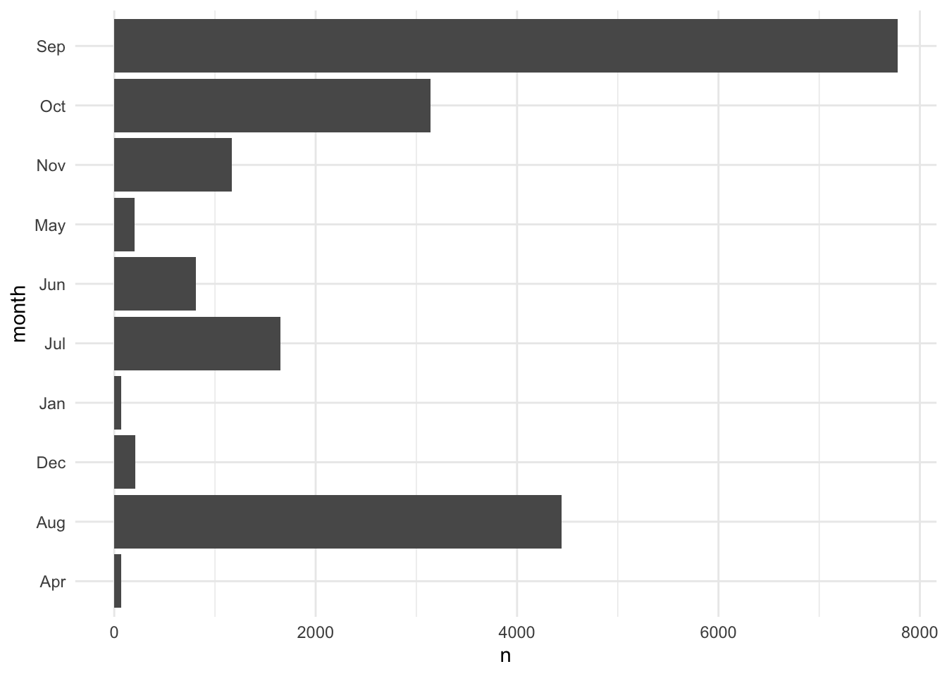

Factors also change the behavior of summary functions like count().

storms |>
  count(month)

# A tibble: 10 × 2
   month     n
   <fct> <int>
 1 Jan      70
 2 Apr      66
 3 May     201
 4 Jun     809
 5 Jul    1651
 6 Aug    4442
 7 Sep    7778
 8 Oct    3138
 9 Nov    1170
10 Dec     212

storms |>
  count(month, .drop = FALSE)

# A tibble: 12 × 2
   month     n
   <fct> <int>
 1 Jan      70
 2 Feb       0
 3 Mar       0
 4 Apr      66
 5 May     201
 6 Jun     809
 7 Jul    1651
 8 Aug    4442
 9 Sep    7778
10 Oct    3138
11 Nov    1170
12 Dec     212

library(forcats) simplifies many common operations on factor vectors.

Changing Order

fct_relevel(), fct_rev(), and fct_reorder() are useful functions for modifying the order of factor variables. Figure 3.2 demonstrates using fct_rev() to flip the order of a categorical axis in ggplot2.

storms |>
  count(month, .drop = FALSE) |>
  ggplot(aes(x = n, y = month)) +
  geom_col()

storms |>
  mutate(month = fct_rev(month)) |>
  count(month, .drop = FALSE) |>
  ggplot(aes(x = n, y = month)) +
  geom_col()

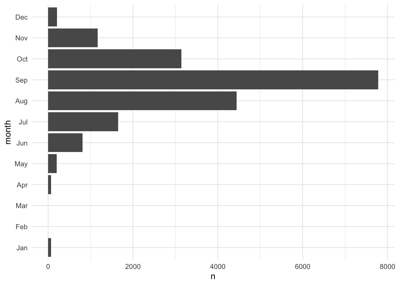
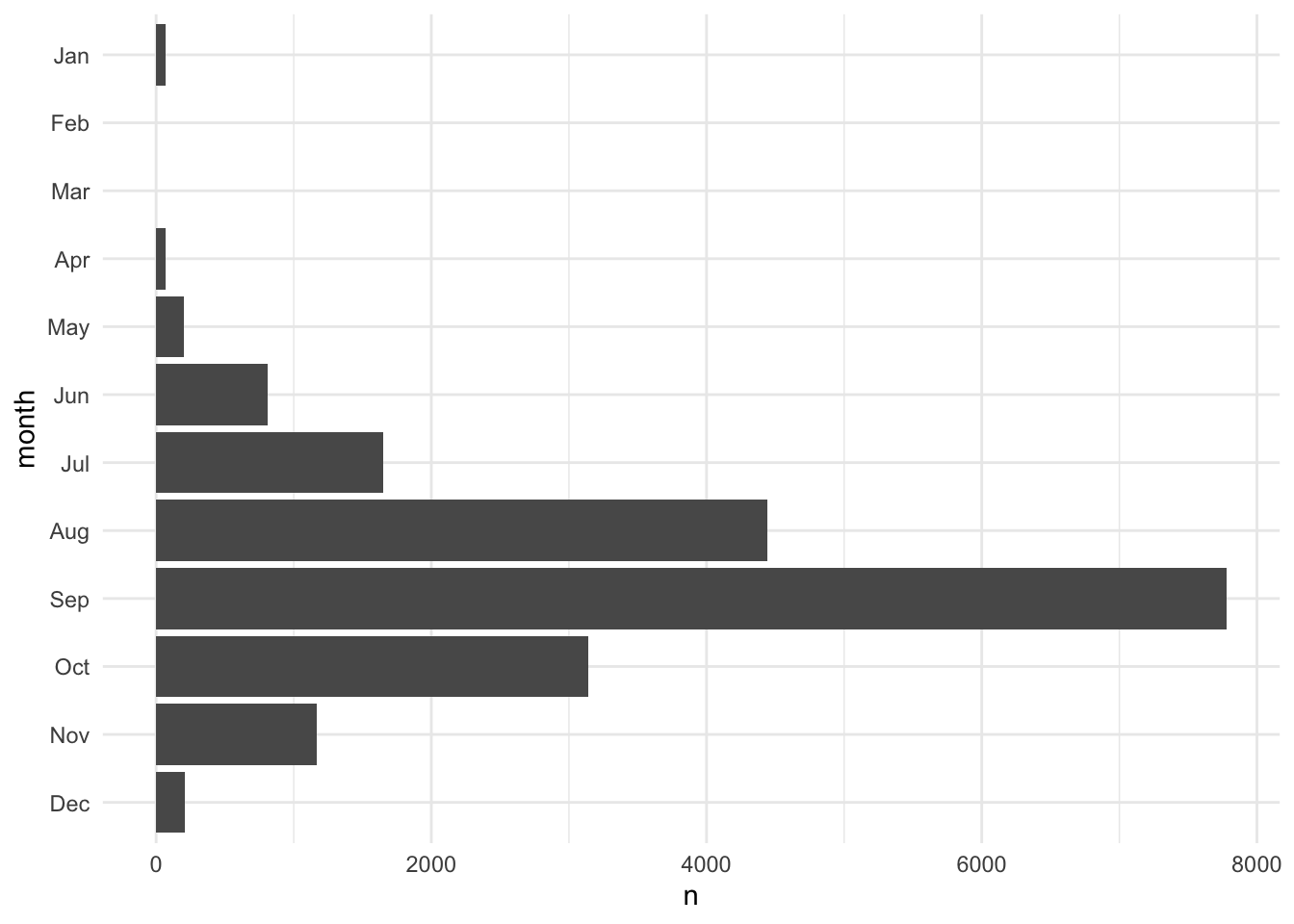
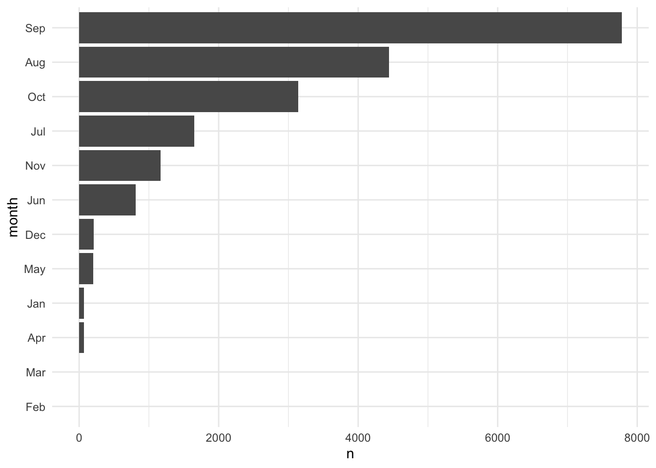
Figure 3.3 orders the factor variable based on the number of observations in each category using fct_reorder(). fct_reorder() can order variables based on more sophisticated summaries than just magnitude. For example, it can order box-and-whisker plots based on the median or even something as arbitrary at the 60th percentile.

storms |>
  count(month, .drop = FALSE) |>
  ggplot(aes(x = n, y = month)) +
  geom_col()

storms |>
  count(month, .drop = FALSE) |>
  mutate(month = fct_reorder(.f = month, .x = n, .fun = median)) |>
  ggplot(aes(x = n, y = month)) +
  geom_col()

Changing Values

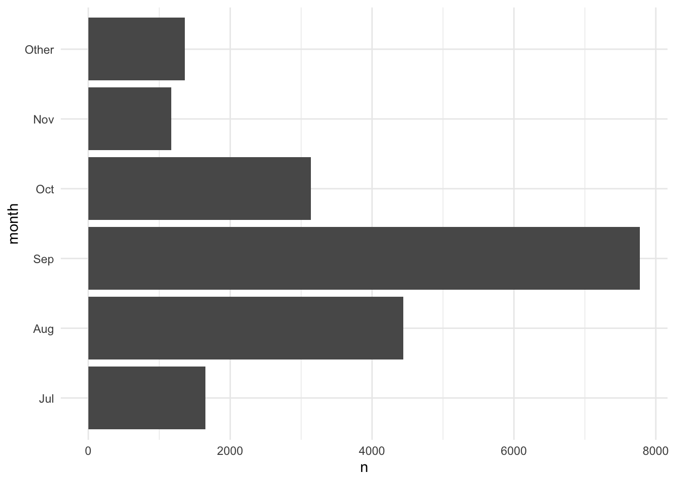
Functions like fct_recode() and fct_lump_min() are useful for changing factor variables. Figure 3.4 combines categories with fewer than 1,000 observations into an "Other" group.

storms |>
  count(month, .drop = FALSE) |>
  ggplot(aes(x = n, y = month)) +
  geom_col()

storms |>
  mutate(month = fct_lump_min(month, min = 1000)) |>  
  count(month, .drop = FALSE) |>
  ggplot(aes(x = n, y = month)) +
  geom_col()

3.4.3 Dates and Date-Times

Check out the lubridate cheat sheet.

There are many ways to store dates.

March 14, 1992
03/14/1992
14/03/1992
14th of March ’92

One way of storing dates is the best. The ISO 8601 date format is an international standard with appealing properties like fixed lengths and self ordering. The format is YYYY-MM-DD.

library(lubridate) has useful functions that will take dates of any format and convert them to the ISO 8601 standard.

library(lubridate)

mdy("March 14, 1992")

[1] "1992-03-14"

mdy("03/14/1992")

[1] "1992-03-14"

dmy("14/03/1992")

[1] "1992-03-14"

dmy("14th of March '92")

[1] "1992-03-14"

These functions return variables of class "Date".

class(mdy("March 14, 1992"))

[1] "Date"

library(lubridate) also contains functions for parsing date times into ISO 8601 standard. Times are slightly trickier because of time zones.

mdy_hms("12/02/2021 1:00:00")

[1] "2021-12-02 01:00:00 UTC"

mdy_hms("12/02/2021 1:00:00", tz = "EST")

[1] "2021-12-02 01:00:00 EST"

mdy_hms("12/02/2021 1:00:00", tz = "America/Chicago")

[1] "2021-12-02 01:00:00 CST"

By default, library(lubridate) will put the date times in Coordinated Universal Time (UTC), which is the successor to Greenwich Mean Time (GMT). I recommend carefully reading the data dictionary if time zones are important for your analysis or if your data cross time zones. This is especially important during time changes (e.g. “spring forward” and “fall back”).

Fortunately, if you encode your dates or date-times correctly, then library(lubridate) will automatically account for time changes, time zones, leap years, leap seconds, and all of the quirks of dates and times.

Exercise 5

dates <- tribble(
  ~date,
  "12/01/1987",
  "12/02/1987",
  "12/03/1987"
)

Create the dates data from above with tribble().
Use mutate() to convert the date column to the ISO 8601 standard (YYYY-MM-DD).

Extracting Components

library(lubridate) contains functions for extracting components from dates like the year, month, day, and weekday. Conisder the follow data set about full moons in Washington, DC in 2023.

full_moons <- tribble(
  ~full_moon,
  "2023-01-06",
  "2023-02-05",
  "2023-03-07",
  "2023-04-06",
  "2023-05-05",
  "2023-06-03",
  "2023-07-03",
  "2023-08-01",
  "2023-08-30",
  "2023-09-29",
  "2023-10-28",
  "2023-11-27",
  "2023-12-26"
) |>
  mutate(full_moon = as_date(full_moon))

Suppose we want to know the weekday of each full moon.

full_moons |>
  mutate(week_day = wday(full_moon, label = TRUE))

# A tibble: 13 × 2
   full_moon  week_day
   <date>     <ord>   
 1 2023-01-06 Fri     
 2 2023-02-05 Sun     
 3 2023-03-07 Tue     
 4 2023-04-06 Thu     
 5 2023-05-05 Fri     
 6 2023-06-03 Sat     
 7 2023-07-03 Mon     
 8 2023-08-01 Tue     
 9 2023-08-30 Wed     
10 2023-09-29 Fri     
11 2023-10-28 Sat     
12 2023-11-27 Mon     
13 2023-12-26 Tue

Math

library(lubridate) easily handles math with dates and date-times. Suppose we want to calculate the number of days since American Independence Day:

today() - as_date("1776-07-04")

Time difference of 90554 days

In this case, subtraction creates an object of class difftime represented in days. We can use the difftimes() function to calculate differences in other units.

difftime(today(), as_date("1776-07-04"), units = "mins")

Time difference of 130397760 mins

Periods

Periods track clock time or a calendar time. We use periods when we set a recurring meetings on a calendar and when we set an alarm to wake up in the morning.

This can lead to some interesting results. Do we always add 365 days when we add 1 year to a date? With periods, this isn’t true. Sometimes we add 366 days during leap years. For example,

start <- as_date("1999-03-14")
end <- start + years(1)

end

[1] "2000-03-14"

end - start

Time difference of 366 days

Durations

Durations track the passage of physical time in exact seconds. Durations are like sand falling into an hourglass. Duration functions start with d like dyears() and dminutes().

start <- as_date("1999-03-14")
end <- start + dyears(1)

end

[1] "2000-03-13 06:00:00 UTC"

Now we always add 365 days, but we see that March 13th is one year after March 14th.

Intervals

Until now, we’ve focused on points in time. Intervals have length and have a starting point and an ending point.

Suppose classes start on August 23rd and proceed every week for a while. Do any of these dates conflict with Georgetown’s fall break?

classes <- as_date("2023-08-23") + weeks(0:15)

fall_break <- interval(as_date("2023-11-22"), as_date("2023-11-26"))

classes %within% fall_break

 [1] FALSE FALSE FALSE FALSE FALSE FALSE FALSE FALSE FALSE FALSE FALSE FALSE
[13] FALSE  TRUE FALSE FALSE

We focused on dates, but many of the same principles hold for date-times.

Exercise 6

Create a date object for your birth date.
Calculate the number of days since your birth date.
Create a vector of your birthdays from your birth date for the next 120 years. Do you use periods or durations?

3.4.4 Missing Data

Missing data are ever present in data analysis. R stores missing values as NA, which are contagious and are fortunately difficult to ignore.

replace_na() is the quickest function to replace missing values. It is a shortcut for a specific instance of if_else().

x <- c(1, NA, 3)

if_else(condition = is.na(x), true = 2, false = x)

[1] 1 2 3

replace_na(x, replace = 2)

[1] 1 2 3

We recommend avoiding arguments like na.rm and using filter() for structurally missing values and replace_na() or imputation for nonresponse. We introduce more sophisticated methods to handle missing data in a later chapter.

Exercise 7

Let’s focus on different data shared by SOI. Now we’ll focus on individual income and tax data by state.

This Excel workbook is a beast. For instance, it isn’t clear how the hierarchy works. I expected all of the rows nested under “Number of returns” to sum up to the number of returns. Unfortunately, the rows are not disjoint. Also, the merged cells for column headers are very difficult to use with programming languages.

Start with 20in01al.xlsx.
Create a tidy data frame with rows 10 through 12 (“Number of single returns”, “Number of joint returns”, and “Number of head of household returns”) disaggregated by “size of adjusted gross income”.

3.5 Conclusion

Key takeaways from this chapter are:

here is a helpful package for reading data, and it is especially helpful when using .Rprojs.
readxl is great for reading excel files into R.
pivot_wider() and pivot_longer() are functions from the tidyr package that are useful for reshaping data into a “tidy” format.
The tidyverse also contains useful package for handing strings (stringr) factors (forecats), and dates (lubridate).

The instinct to include these comments is good. The execution is poor because it creates big headaches for people using programming languages. We suggest using a data dictionary instead.↩︎
This example uses regular expressions (regex). Visit R4DS (2e) for a review of regex.↩︎

3.1 Review

3.2 Import

3.2.1 library(here)

3.2.2 library(readxl)

3.3 Tidy

Tidying Example 1

Tidying Example 2

Tidying Example 3

Tidying Example 4

3.4 Transform

3.4.1 Strings

Detecting Matches

Subsetting Strings

Managing Lengths

Modifying Strings

3.4.2 Factors {sec-factors}

Factor Basics

Changing Order

Changing Values

3.4.3 Dates and Date-Times

Extracting Components

Math

Periods

Durations

Intervals

3.4.4 Missing Data

3.5 Conclusion

3.2.1 `library(here)`

3.2.2 `library(readxl)`